Tài liệu Báo cáo khoa học: "Discovering Global Patterns in Linguistic Networks through Spectral Analysis: A Case Study of the Consonant Inventories" pdf

Proceedings of the 12th Conference of the European Chapter of the ACL, pages 585–593,
Athens, Greece, 30 March – 3 April 2009.
c
2009 Association for Computational Linguistics
Discovering Global Patterns in Linguistic Networks through
Spectral Analysis: A Case Study of the Consonant Inventories
Animesh Mukherjee
∗
Indian Institute of Technology, Kharagpur

Monojit Choudhury and Ravi Kannan
Microsoft Research India
{monojitc,kannan}@microsoft.com
Abstract
Recent research has shown that language
and the socio-cognitive phenomena asso-
ciated with it can be aptly modeled and
visualized through networks of linguistic
entities. However, most of the existing
works on linguistic networks focus only
on the local properties of the networks.
This study is an attempt to analyze the
structure of languages via a purely struc-
tural technique, namely spectral analysis,
which is ideally suited for discovering the
global correlations in a network. Appli-
cation of this technique to PhoNet, the
co-occurrence network of consonants, not
only reveals several natural linguistic prin-
ciples governing the structure of the con-
sonant inventories, but is also able to quan-

tify their relative importance. We believe
that this powerful technique can be suc-
cessfully applied, in general, to study the
structure of natural languages.
1 Introduction
Language and the associated socio-cognitive phe-
nomena can be modeled as networks, where the
nodes correspond to linguistic entities and the
edges denote the pairwise interaction or relation-
ship between these entities. The study of lin-
guistic networks has been quite popular in the re-
cent times and has provided us with several in-
teresting insights into the nature of language (see
Choudhury and Mukherjee (to appear) for an ex-
tensive survey). Examples include study of the
WordNet (Sigman and Cecchi, 2002), syntactic
dependency network of words (Ferrer-i-Cancho,
2005) and network of co-occurrence of conso-
nants in sound inventories (Mukherjee et al., 2008;
Mukherjee et al., 2007).
∗
This research has been conducted during the author’s in-
ternship at Microsoft Research India.
Most of the existing studies on linguistic net-
works, however, focus only on the local structural
properties such as the degree and clustering coef-
ficient of the nodes, and shortest paths between
pairs of nodes. On the other hand, although it is
a well known fact that the spectrum of a network
can provide important information about its global

structure, the use of this powerful mathematical
machinery to infer global patterns in linguistic net-
works is rarely found in the literature. Note that
spectral analysis, however, has been successfully
employed in the domains of biological and social
networks (Farkas et al., 2001; Gkantsidis et al.,
2003; Banerjee and Jost, 2007). In the context of
linguistic networks, (Belkin and Goldsmith, 2002)
is the only work we are aware of that analyzes the
eigenvectors to obtain a two dimensional visualize
of the network. Nevertheless, the work does not
study the spectrum of the graph.
The aim of the present work is to demonstrate
the use of spectral analysis for discovering the
global patterns in linguistic networks. These pat-
terns, in turn, are then interpreted in the light of ex-
isting linguistic theories to gather deeper insights
into the nature of the underlying linguistic phe-
nomena. We apply this rather generic technique
to find the principles that are responsible for shap-
ing the consonant inventories, which is a well re-
searched problem in phonology since 1931 (Tru-
betzkoy, 1931; Lindblom and Maddieson, 1988;
Boersma, 1998; Clements, 2008). The analysis
is carried out on a network defined in (Mukherjee
et al., 2007), where the consonants are the nodes
and there is an edge between two nodes u and v
if the consonants corresponding to them co-occur
in a language. The number of times they co-occur
across languages define the weight of the edge. We

explain the results obtained from the spectral anal-
ysis of the network post-facto using three linguis-
tic principles. The method also automatically re-
veals the quantitative importance of each of these
585
principles.
It is worth mentioning here that earlier re-
searchers have also noted the importance of the
aforementioned principles. However, what was
not known was how much importance one should
associate with each of these principles. We also
note that the technique of spectral analysis neither
explicitly nor implicitly assumes that these princi-
ples exist or are important, but deduces them auto-
matically. Thus, we believe that spectral analysis
is a promising approach that is well suited to the
discovery of linguistic principles underlying a set
of observations represented as a network of enti-
ties. The fact that the principles “discovered” in
this study are already well established results adds
to the credibility of the method. Spectral analysis
of large linguistic networks in the future can possi-
bly reveal hitherto unknown universal principles.
The rest of the paper is organized as follows.
Sec. 2 introduces the technique of spectral anal-
ysis of networks and illustrates some of its ap-
plications. The problem of consonant inventories
and how it can be modeled and studied within the
framework of linguistic networks are described in
Sec. 3. Sec. 4 presents the spectral analysis of

the consonant co-occurrence network, the obser-
vations and interpretations. Sec. 5 concludes by
summarizing the work and the contributions and
listing out future research directions.
2 A Primer to Spectral Analysis
Spectral analysis
1
is a powerful tool capable of
revealing the global structural patterns underly-
ing an enormous and complicated environment
of interacting entities. Essentially, it refers to
the systematic study of the eigenvalues and the
eigenvectors of the adjacency matrix of the net-
work of these interacting entities. Here we shall
briefly review the basic concepts involved in spec-
tral analysis and describe some of its applications
(see (Chung, 1994; Kannan and Vempala, 2008)
for details).
A network or a graph consisting of n nodes (la-
beled as 1 through n) can be represented by a n×n
square matrix A, where the entry a
ij
represents the
weight of the edge from node i to node j. A, which
is known as the adjacency matrix, is symmetric for
an undirected graph and have binary entries for an
1
The term spectral analysis is also used in the context of
signal processing, where it refers to the study of the frequency
spectrum of a signal.

unweighted graph. λ is an eigenvalue of A if there
is an n-dimensional vector x such that
Ax = λx
Any real symmetric matrix A has n (possibly non-
distinct) eigenvalues λ
0
≤ λ
1
≤ . . . ≤ λ
n−1
, and
corresponding n eigenvectors that are mutually or-
thogonal. The spectrum of a graph is the set of the
distinct eigenvalues of the graph and their corre-
sponding multiplicities. It is usually represented
as a plot with the eigenvalues in x-axis and their
multiplicities plotted in the y-axis.
The spectrum of real and random graphs dis-
play several interesting properties. Banerjee and
Jost (2007) report the spectrum of several biologi-
cal networks that are significantly different from
the spectrum of artificially generated graphs
2
.
Spectral analysis is also closely related to Prin-
cipal Component Analysis and Multidimensional
Scaling. If the first few (say d) eigenvalues of a
matrix are much higher than the rest of the eigen-
values, then it can be concluded that the rows of
the matrix can be approximately represented as

linear combinations of d orthogonal vectors. This
further implies that the corresponding graph has
a few motifs (subgraphs) that are repeated a large
number of time to obtain the global structure of
the graph (Banerjee and Jost, to appear).
Spectral properties are representative of an n-
dimensional average behavior of the underlying
system, thereby providing considerable insight
into its global organization. For example, the prin-
cipal eigenvector (i.e., the eigenvector correspond-
ing to the largest eigenvalue) is the direction in
which the sum of the square of the projections
of the row vectors of the matrix is maximum. In
fact, the principal eigenvector of a graph is used to
compute the centrality of the nodes, which is also
known as PageRank in the context of WWW. Sim-
ilarly, the second eigen vector component is used
for graph clustering.
In the next two sections we describe how spec-
tral analysis can be applied to discover the orga-
nizing principles underneath the structure of con-
sonant inventories.
2
Banerjee and Jost (2007) report the spectrum of the
graph’s Laplacian matrix rather than the adjacency matrix.
It is increasingly popular these days to analyze the spectral
properties of the graph’s Laplacian matrix. However, for rea-
sons explained later, here we will be conduct spectral analysis
of the adjacency matrix rather than its Laplacian.
586

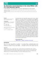
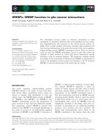
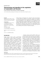
Figure 1: Illustration of the nodes and edges of PlaNet and PhoNet along with their respective adjacency
matrix representations.
3 Consonant Co-occurrence Network
The most basic unit of human languages are the
speech sounds. The repertoire of sounds that make
up the sound inventory of a language are not cho-
sen arbitrarily even though the speakers are ca-
pable of producing and perceiving a plethora of
them. In contrast, these inventories show excep-
tionally regular patterns across the languages of
the world, which is in fact, a common point of
consensus in phonology. Right from the begin-
ning of the 20
th
century, there have been a large
number of linguistically motivated attempts (Tru-
betzkoy, 1969; Lindblom and Maddieson, 1988;
Boersma, 1998; Clements, 2008) to explain the
formation of these patterns across the consonant
inventories. More recently, Mukherjee and his col-
leagues (Choudhury et al., 2006; Mukherjee et al.,
2007; Mukherjee et al., 2008) studied this problem
in the framework of complex networks. Since here
we shall conduct a spectral analysis of the network
defined in Mukherjee et al. (2007), we briefly sur-
vey the models and the important results of their
work.
Choudhury et al. (2006) introduced a bipartite
network model for the consonant inventories. For-
mally, a set of consonant inventories is represented

as a graph G = V
L
, V
C
, E
lc
, where the nodes in
one partition correspond to the languages (V
L
) and
that in the other partition correspond to the conso-
nants (V
C
). There is an edge (v
l
, v
c
) between a
language node v
l
∈ V
L
(representing the language
l) and a consonant node v
c
∈ V
C
(representing the
consonant c) iff the consonant c is present in the
inventory of the language l. This network is called

the Phoneme-Language Network or PlaNet and
represent the connections between the language
and the consonant nodes through a 0-1 matrix A
as shown by a hypothetical example in Fig. 1. Fur-
ther, in (Mukherjee et al., 2007), the authors define
the Phoneme-Phoneme Network or PhoNet as the
one-mode projection of PlaNet onto the consonant
nodes, i.e., a network G = V
C
, E
cc

, where the
nodes are the consonants and two nodes v
c
and
v
c

are linked by an edge with weight equal to the
number of languages in which both c and c

occur
together. In other words, PhoNet can be expressed
as a matrix B (see Fig. 1) such that B = AA
T
−D
where D is a diagonal matrix with its entries cor-
responding to the frequency of occurrence of the
consonants. Similarly, we can also construct the

one-mode projection of PlaNet onto the language
nodes (which we shall refer to as the Language-
Language Graph or LangGraph) can be expressed
as B

= A
T
A −D

, where D

is a diagonal ma-
trix with its entries corresponding to the size of the
consonant inventories for each language.
The matrix A and hence, B and B

have been
constructed from the UCLA Phonological Seg-
ment Inventory Database (UPSID) (Maddieson,
1984) that hosts the consonant inventories of 317
languages with a total of 541 consonants found
across them. Note that, UPSID uses articulatory
587
features to describe the consonants and assumes
these features to be binary-valued, which in turn
implies that every consonant can be represented
by a binary vector. Later on, we shall use this rep-
resentation for our experiments.
By construction, we have |V
L

| = 317, |V
C
| =
541, |E
lc
| = 7022, and |E
cc

| = 30412. Conse-
quently, the order of the matrix A is 541 × 317
and that of the matrix B

is 541 × 541. It has been
found that the degree distribution of both PlaNet
and PhoNet roughly indicate a power-law behavior
with exponential cut-offs towards the tail (Choud-
hury et al., 2006; Mukherjee et al., 2007). Further-
more, PhoNet is also characterized by a very high
clustering coefficient. The topological properties
of the two networks and the generative model
explaining the emergence of these properties are
summarized in (Mukherjee et al., 2008). However,
all the above properties are useful in characteriz-
ing the local patterns of the network and provide
very little insight about its global structure.
4 Spectral Analysis of PhoNet
In this section we describe the procedure and re-
sults of the spectral analysis of PhoNet. We begin
with computation of the spectrum of PhoNet. Af-
ter the analysis of the spectrum, we systematically

investigate the top few eigenvectors of PhoNet
and attempt to characterize their linguistic signif-
icance. In the process, we also analyze the corre-
sponding eigenvectors of LanGraph that helps us
in characterizing the properties of languages.
4.1 Spectrum of PhoNet
Using a simple Matlab script we compute the
spectrum (i.e., the list of eignevalues along with
their multiplicities) of the matrix B correspond-
ing to PhoNet. Fig. 2(a) shows the spectral plot,
which has been obtained through binning
3
with a
fixed bin size of 20. In order to have a better visu-
alization of the spectrum, in Figs. 2(b) and (c) we
further plot the top 50 (absolute) eigenvalues from
the two ends of the spectrum versus the index rep-
resenting their sorted order in doubly-logarithmic
scale. Some of the important observations that one
can make from these results are as follows.
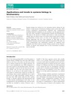
First, the major bulk of the eigenvalues are con-
centrated at around 0. This indicates that though
3
Binning is the process of dividing the entire range of a
variable into smaller intervals and counting the number of
observations within each bin or interval. In fixed binning, all
the intervals are of the same size.
the order of B is 541 × 541, its numerical rank is
quite low. Second, there are at least a few very
large eigenvalues that dominate the entire spec-

trum. In fact, 89% of the spectrum, or the square
of the Frobenius norm, is occupied by the princi-
pal (i.e., the topmost) eigenvalue, 92% is occupied
by the first and the second eigenvalues taken to-
gether, while 93% is occupied by the first three
taken together. The individual contribution of the
other eigenvalues to the spectrum is significantly
lower than that of the top three. Third, the eigen-
values on either ends of the spectrum tend to decay
gradually, mostly indicating a power-law behavior.
The power-law exponents at the positive and the
negative ends are -1.33 (the R
2
value of the fit is
0.98) and -0.88 (R
2
∼ 0.92) respectively.
The numerically low rank of PhoNet suggests
that there are certain prototypical structures that
frequently repeat themselves across the consonant
inventories, thereby, increasing the number of 0
eigenvalues to a large extent. In other words, all
the rows of the matrix B (i.e., the inventories) can
be expressed as the linear combination of a few
independent row vectors, also known as factors.
Furthermore, the fact that the principal eigen-
value constitutes 89% of the Frobenius norm of the
spectrum implies that there exist one very strong
organizing principle which should be able to ex-
plain the basic structure of the inventories to a very

good extent. Since the second and third eigen-
values are also significantly larger than the rest
of the eigenvalues, one should expect two other
organizing principles, which along with the basic
principle, should be able to explain, (almost) com-
pletely, the structure of the inventories. In order
to “discover” these principles, we now focus our
attention to the first three eigenvectors of PhoNet.
4.2 The First Eigenvector of PhoNet
Fig. 2(d) shows the first eigenvector component
for each consonant node versus its frequency of
occurrence across the language inventories (i.e., its
degree in PlaNet). The figure clearly indicates that
the two are highly correlated (r = 0.99), which in
turn means that 89% of the spectrum and hence,
the organization of the consonant inventories, can
be explained to a large extent by the occurrence
frequency of the consonants. The question arises:
Does this tell us something special about the struc-
ture of PhoNet or is it always the case for any sym-
metric matrix that the principal eigenvector will
588
Figure 2: Eigenvalues and eigenvectors of B. (a) Binned distribution of the eigenvalues (bin size = 20)
versus their multiplicities. (b) the top 50 (absolute) eigenvalues from the positive end of the spectrum and
their ranks. (c) Same as (b) for the negative end of the spectrum. (d), (e) and (f) respectively represents
the first, second and the third eigenvector components versus the occurrence frequency of the consonants.
be highly correlated with the frequency? We as-
sert that the former is true, and indeed, the high
correlation between the principal eigenvector and
the frequency indicates high “proportionate co-

occurrence” - a term which we will explain.
To see this, consider the following 2n ×2n ma-
trix X
X =








0 M
1
0 0 0 . . .
M
1
0 0 0 0 . . .
0 0 0 M
2
0 . . .
0 0 M
2
0 0 . . .
.
.
.
.
.
.

.
.
.
.
.
.
.
.
.
.
.
.








where X
i,i+1
= X
i+1,i
= M
(i+1)/2
for all odd
i and 0 elsewhere. Also, M
1
> M

2
> . . . >
M
n
≥ 1. Essentially, this matrix represents a
graph which is a collection of n disconnected
edges, each having weights M
1
, M
2
, and so on.
It is easy to see that the principal eigenvector of
this matrix is (1/
√
2, 1/
√
2, 0, 0, . . . , 0)

, which
of course is very different from the frequency vec-
tor: (M
1
, M
1
, M
2
, M
2
, . . . , M
n

, M
n
)

.
At the other extreme, consider an n × n ma-
trix X with X
i,j
= Cf
i
f
j
for some vector f =
(f
1
, f
2
, . . . f
n
)

that represents the frequency of
the nodes and a normalization constant C. This is
what we refer to as ”proportionate co-occurrence”
because the extent of co-occurrence between the
nodes i and j (which is X
i,j
or the weight of the
edge between i and j) is exactly proportionate to
the frequencies of the two nodes. The principal

eigenvector in this case is f itself, and thus, corre-
lates perfectly with the frequencies. Unlike this
hypothetical matrix X, PhoNet has all 0 entries
in the diagonal. Nevertheless, this perturbation,
which is equivalent to subtracting f
2
i
from the i
th
diagonal, seems to be sufficiently small to preserve
the “proportionate co-occurrence” behavior of the
adjacency matrix thereby resulting into a high cor-
relation between the principal eigenvector compo-
nent and the frequencies.
On the other hand, to construct the Lapla-
cian matrix, we would have subtracted f
i

n
j=1
f
j
from the i
th
diagonal entry, which is a much
larger quantity than f
2
i
. In fact, this operation
would have completely destroyed the correlation

between the frequency and the principal eigen-
vector component because the eigenvector corre-
sponding to the smallest
4
eigenvalue of the Lapla-
cian matrix is [1, 1, . . . , 1]

.
Since the first eigenvector of B is perfectly cor-
4
The role played by the top eigenvalues and eigenvectors
in the spectral analysis of the adjacency matrix is compara-
ble to that of the smallest eigenvalues and the corresponding
eigenvectors of the Laplacian matrix (Chung, 1994)
589
related with the frequency of occurrence of the
consonants across languages it is reasonable to
argue that there is a universally observed innate
preference towards certain consonants. This pref-
erence is often described through the linguistic
concept of markedness, which in the context of
phonology tells us that the substantive conditions
that underlie the human capacity of speech pro-
duction and perception renders certain consonants
more favorable to be included in the inventory than
some other consonants (Clements, 2008). We ob-
serve that markedness plays a very important role
in shaping the global structure of the consonant in-
ventories. In fact, if we arrange the consonants in a
non-increasing order of the first eigenvector com-

ponents (which is equivalent to increasing order
of statistical markedness), and compare the set of
consonants present in an inventory of size s with
that of the first s entries from this hierarchy, we
find that the two are, on an average, more than
50% similar. This figure is surprisingly high be-
cause, in spite of the fact that ∀
s
s 
541
2
, on an
average
s
2
consonants in an inventory are drawn
from the first s entries of the markedness hierarchy
(a small set), whereas the rest
s
2
are drawn from the
remaining (541 − s) entries (a much larger set).
The high degree of proportionate co-occurrence
in PhoNet implied by this high correlation be-
tween the principal eigenvector and frequency fur-
ther indicates that the innate preference towards
certain phonemes is independent of the presence
of other phonemes in the inventory of a language.
4.3 The Second Eigenvector of PhoNet
Fig. 2(e) shows the second eigenvector component

for each node versus their occurrence frequency. It
is evident from the figure that the consonants have
been clustered into three groups. Those that have
a very low or a very high frequency club around 0
whereas, the medium frequency zone has clearly
split into two parts. In order to investigate the ba-
sis for this split we carry out the following experi-
ment.
Experiment I
(i) Remove all consonants whose frequency of oc-
currence across the inventories is very low (< 5).
(ii) Denote the absolute maximum value of the
positive component of the second eigenvector as
MAX
+
and the absolute maximum value of the
negative component as MAX
−
. If the absolute
value of a positive component is less than 15% of
MAX
+
then assign a neutral class to the corre-
sponding consonant; else assign it a positive class.
Denote the set of consonants in the positive class
by C
+
. Similarly, if the absolute value of a nega-
tive component is less than 15% of M AX
−

then
assign a neutral class to the corresponding conso-
nant; else assign it a negative class. Denote the set
of consonants in the negative class by C
−
.
(iii) Using the above training set of the classified
consonants (represented as boolean feature vec-
tors) learn a decision tree (C4.5 algorithm (Quin-
lan, 1993)) to determine the features that are re-
sponsible for the split of the medium frequency
zone into the negative and the positive classes.
Fig. 3(a) shows the decision rules learnt from
the above training set. It is clear from these rules
that the split into C
−
and C
+
has taken place
mainly based on whether the consonants have
the combined “dental alveolar” feature (negative
class) or the “dental” and the “alveolar” features
separately (positive class). Such a combined fea-
ture is often termed ambiguous and its presence in
a particular consonant c of a language l indicates
that the speakers of l are unable to make a distinc-
tion as to whether c is articulated with the tongue
against the upper teeth or the alveolar ridge. In
contrast, if the features are present separately then
the speakers are capable of making this distinc-

tion. In fact, through the following experiment,
we find that the consonant inventories of almost
all the languages in UPSID get classified based on
whether they preserve this distinction or not.
Experiment II
(i) Construct B

= A
T
A – D

(i.e., the adjacency
matrix of LangGraph).
(ii) Compute the second eigenvector of B

. Once
again, the positive and the negative components
split the languages into two distinct groups L
+
and
L
−
respectively.
(iii) For each language l ∈ L
+
count the num-
ber of consonants in C
+
that occur in l. Sum up
the counts for all the languages in L

+
and nor-
malize this sum by |L
+
||C
+
|. Similarly, perform
the same step for the pairs (L
+
,C
−
), (L
−
,C
+
) and
(L
−
,C
−
).
From the above experiment, the values obtained
for the pairs (i) (L
+
,C
+
), (L
+
,C
−

) are 0.35, 0.08
respectively, and (ii) (L
−
,C
+
), (L
−
,C
−
) are 0.07,
0.32 respectively. This immediately implies that
almost all the languages in L
+
preserve the den-
tal/alveolar distinction while those in L
−
do not.
590
Figure 3: Decision rules obtained from the study of (a) the second, and (b) the third eigenvectors. The
classification errors for both (a) and (b) are less than 15%.
4.4 The Third Eigenvector of PhoNet
We next investigate the relationship between the
third eigenvector components of B and the occur-
rence frequency of the consonants (Fig. 2(f)). The
consonants are once again found to get clustered
into three groups, though not as clearly as in the
previous case. Therefore, in order to determine the
basis of the split, we repeat experiments I and II.
Fig. 3(b) clearly indicates that in this case the con-
sonants in C

+
lack the complex features that are
considered difficult for articulation. On the other
hand, the consonants in C
−
are mostly composed
of such complex features. The values obtained for
the pairs (i) (L
+
,C
+
), (L
+
,C
−
) are 0.34, 0.06 re-
spectively, and (ii) (L
−
,C
+
), (L
−
,C
−
) are 0.19,
0.18 respectively. This implies that while there is
a prevalence of the consonants from C
+
in the lan-
guages of L

+
, the consonants from C
−
are almost
absent. However, there is an equal prevalence of
the consonants from C
+
and C
−
in the languages
of L
−
. Therefore, it can be argued that the pres-
ence of the consonants from C
−
in a language can
(phonologically) imply the presence of the conso-
nants from C
+
, but not vice versa. We do not find
any such aforementioned pattern for the fourth and
the higher eigenvector components.
4.5 Control Experiment
As a control experiment we generated a set of ran-
dom inventories and carried out the experiments
I and II on the adjacency matrix, B
R
, of the ran-
dom version of PhoNet. We construct these in-
ventories as follows. Let the frequency of occur-

rence for each consonant c in UPSID be denoted
by f
c
. Let there be 317 bins each corresponding to
a language in UPSID. f
c
bins are then chosen uni-
formly at random and the consonant c is packed
into these bins. Thus the consonant inventories
of the 317 languages corresponding to the bins
are generated. Note that this method of inventory
construction leads to proportionate co-occurrence.
Consequently, the first eigenvector components of
B
R
are highly correlated to the occurrence fre-
quency of the consonants. However, the plots of
the second and the third eigenvector components
versus the occurrence frequency of the consonants
indicate absolutely no pattern thereby, resulting in
a large number of decision rules and very high
classification errors (upto 50%).
591
5 Discussion and Conclusion
Are there any linguistic inferences that can be
drawn from the results obtained through the
study of the spectral plot and the eigenvectors of
PhoNet? In fact, one can correlate several phono-
logical theories to the aforementioned observa-
tions, which have been construed by the past re-

searchers through very specific studies.
One of the most important problems in defin-
ing a feature-based classificatory system is to de-
cide when a sound in one language is different
from a similar sound in another language. Ac-
cording to Ladefoged (2005) “two sounds in dif-
ferent languages should be considered as distinct
if we can point to a third language in which the
same two sounds distinguish words”. The den-
tal versus alveolar distinction that we find to be
highly instrumental in splitting the world’s lan-
guages into two different groups (i.e., L
+
and L
−
obtained from the analysis of the second eigen-
vectors of B and B

) also has a strong classifi-
catory basis. It may well be the case that cer-
tain categories of sounds like the dental and the
alveolar sibilants are not sufficiently distinct to
constitute a reliable linguistic contrast (see (Lade-
foged, 2005) for reference). Nevertheless, by al-
lowing the possibility for the dental versus alveo-
lar distinction, one does not increase the complex-
ity or introduce any redundancy in the classifica-
tory system. This is because, such a distinction
is prevalent in many other sounds, some of which
are (a) nasals in Tamil (Shanmugam, 1972) and

Malayalam (Shanmugam, 1972; Ladefoged and
Maddieson, 1996), (b) laterals in Albanian (Lade-
foged and Maddieson, 1996), and (c) stops in cer-
tain dialectal variations of Swahili (Hayward et al.,
1989). Therefore, it is sensible to conclude that the
two distinct groups L
+
and L
−
induced by our al-
gorithm are true representatives of two important
linguistic typologies.
The results obtained from the analysis of the
third eigenvectors of B and B

indicate that im-
plicational universals also play a crucial role in
determining linguistic typologies. The two ty-
pologies that are predominant in this case con-
sist of (a) languages using only those sounds that
have simple features (e.g., plosives), and (b) lan-
guages using sounds with complex features (e.g.,
lateral, ejectives, and fricatives) that automatically
imply the presence of the sounds having sim-
ple features. The distinction between the simple
and complex phonological features is a very com-
mon hypothesis underlying the implicational hier-
archy and the corresponding typological classifi-
cation (Clements, 2008). In this context, Locke
and Pearson (1992) remark that “Infants heavily

favor stop consonants over fricatives, and there
are languages that have stops and no fricatives but
no languages that exemplify the reverse pattern.
[Such] ‘phonologically universal’ patterns, which
cut across languages and speakers are, in fact, the
phonetic properties of Homo sapiens.” (as quoted
in (Vallee et al., 2002)).
Therefore, it turns out that the methodology pre-
sented here essentially facilitates the induction of
linguistic typologies. Indeed, spectral analysis de-
rives, in a unified way, the importance of these
principles and at the same time quantifies their ap-
plicability in explaining the structural patterns ob-
served across the inventories. In this context, there
are at least two other novelties of this work. The
first novelty is in the systematic study of the spec-
tral plots (i.e., the distribution of the eigenvalues),
which is in general rare for linguistic networks,
although there have been quite a number of such
studies in the domain of biological and social net-
works (Farkas et al., 2001; Gkantsidis et al., 2003;
Banerjee and Jost, 2007). The second novelty is
in the fact that there is not much work in the com-
plex network literature that investigates the nature
of the eigenvectors and their interactions to infer
the organizing principles of the system represented
through the network.
To summarize, spectral analysis of the com-
plex network of speech sounds is able to provide
a holistic as well as quantitative explanation of

the organizing principles of the sound inventories.
This scheme for typology induction is not depen-
dent on the specific data set used as long as it is
representative of the real world. Thus, we believe
that the scheme introduced here can be applied as
a generic technique for typological classifications
of phonological, syntactic and semantic networks;
each of these are equally interesting from the per-
spective of understanding the structure and evolu-
tion of human language, and are topics of future
research.
Acknowledgement
We would like to thank Kalika Bali for her valu-
able inputs towards the linguistic analysis.
592
References
A. Banerjee and J. Jost. 2007. Spectral plots and the
representation and interpretation of biological data.
Theory in Biosciences, 126(1):15–21.
A. Banerjee and J. Jost. to appear. Graph spectra as a
systematic tool in computational biology. Discrete
Applied Mathematics.
M. Belkin and J. Goldsmith. 2002. Using eigenvectors
of the bigram graph to infer morpheme identity. In
Proceedings of the ACL-02 Workshop on Morpho-
logical and Phonological Learning, pages 41–47.
Association for Computational Linguistics.
P. Boersma. 1998. Functional Phonology. The Hague:
Holland Academic Graphics.
M. Choudhury and A. Mukherjee. to appear. The

structure and dynamics of linguistic networks. In
N. Ganguly, A. Deutsch, and A. Mukherjee, editors,
Dynamics on and of Complex Networks: Applica-
tions to Biology, Computer Science, Economics, and
the Social Sciences. Birkhauser.
M. Choudhury, A. Mukherjee, A. Basu, and N. Gan-
guly. 2006. Analysis and synthesis of the distribu-
tion of consonants over languages: A complex net-
work approach. In COLING-ACL’06, pages 128–
135.
F. R. K. Chung. 1994. Spectral Graph Theory. Num-
ber 2 in CBMS Regional Conference Series in Math-
ematics. American Mathematical Society.
G. N. Clements. 2008. The role of features in speech
sound inventories. In E. Raimy and C. Cairns, edi-
tors, Contemporary Views on Architecture and Rep-
resentations in Phonological Theory. Cambridge,
MA: MIT Press.
E. J. Farkas, I. Derenyi, A. -L. Barab
´
asi, and T. Vic-
seck. 2001. Real-world graphs: Beyond the semi-
circle law. Phy. Rev. E, 64:026704.
R. Ferrer-i-Cancho. 2005. The structure of syntac-
tic dependency networks: Insights from recent ad-
vances in network theory. In Levickij V. and Altm-
man G., editors, Problems of quantitative linguistics,
pages 60–75.
C. Gkantsidis, M. Mihail, and E. Zegura. 2003.
Spectral analysis of internet topologies. In INFO-

COM’03, pages 364–374.
K. M. Hayward, Y. A. Omar, and M. Goesche. 1989.
Dental and alveolar stops in Kimvita Swahili: An
electropalatographic study. African Languages and
Cultures, 2(1):51–72.
R. Kannan and S. Vempala. 2008. Spec-
tral Algorithms. Course Lecture Notes:
/>P. Ladefoged and I. Maddieson. 1996. Sounds of the
Worlds Languages. Oxford: Blackwell.
P. Ladefoged. 2005. Features and parameters for
different purposes. In Working Papers in Phonet-
ics, volume 104, pages 1–13. Dept. of Linguistics,
UCLA.
B. Lindblom and I. Maddieson. 1988. Phonetic univer-
sals in consonant systems. In M. Hyman and C. N.
Li, editors, Language, Speech, and Mind, pages 62–
78.
J. L. Locke and D. M. Pearson. 1992. Vocal learn-
ing and the emergence of phonological capacity. A
neurobiological approach. In Phonological devel-
opment. Models, Research, Implications, pages 91–
129. York Press.
I. Maddieson. 1984. Patterns of Sounds. Cambridge
University Press.
A. Mukherjee, M. Choudhury, A. Basu, and N. Gan-
guly. 2007. Modeling the co-occurrence principles
of the consonant inventories: A complex network
approach. Int. Jour. of Mod. Phys. C, 18(2):281–
295.
A. Mukherjee, M. Choudhury, A. Basu, and N. Gan-

guly. 2008. Modeling the structure and dynamics of
the consonant inventories: A complex network ap-
proach. In COLING-08, pages 601–608.
J. R. Quinlan. 1993. C4.5: Programs for Machine
Learning. Morgan Kaufmann.
S. V. Shanmugam. 1972. Dental and alveolar nasals in
Dravidian. In Bulletin of the School of Oriental and
African Studies, volume 35, pages 74–84. University
of London.
M. Sigman and G. A. Cecchi. 2002. Global organi-
zation of the wordnet lexicon. Proceedings of the
National Academy of Science, 99(3):1742–1747.
N. Trubetzkoy. 1931. Die phonologischen systeme.
TCLP, 4:96–116.
N. Trubetzkoy. 1969. Principles of Phonology. Uni-
versity of California Press, Berkeley.
N. Vallee, L J Boe, J. L. Schwartz, P. Badin, and
C. Abry. 2002. The weight of phonetic substance in
the structure of sound inventories. ZASPiL, 28:145–
168.
593