Integral and its application

THAI NGUYEN UNIVERSITY OF EDUCATION
MATHEMATICS
----------

PROBLEM SEMINAR
PROBLEM: Integral

and its application

Supervisors: NGUYEN VAN THIN
Group : 3
Class: Mathematical analysis I

June, 2022


TABLE OF CONTENTS
INTRODUCTION OF PRINCIPLES – ANALYSIS ................................................................... 5
PRINCIPLES AND DIFFERENTIAL ANALYSIS

5

Define

5

Nature

5

DEFINITION ANALYSIS

5

Define

5

Nature

6

ANALYSIS METHODS

6

Primitives of some basic functions

6

Integral Calculation Methods

7

Sub-conclusion

9

FEATURES ON THE BIRTH AND DEVELOPMENT OF THE THEORY OF ANALYSIS10
10
1. HISTORY ANALYSIS

11
2. ANALYSIS APPLICATION
APPLICATIONS OF DEFINITION ANALYSIS………………………………………………12
1. GEOLOGICAL APPLICATIONS OF DEFINITIONAL ANALYSIS
A. General diagram using integrals

12

12

B. Area of flat figure
C. Bow length

13
18


2. Algebraic Applications of DEFINITIONAL ANALYSIS

20

A. Integral inequality

20

B. Integral applications prove the inequality

20

CONCLUSION………………………………………………………………………………….21

The outline of primitives - integrals
1. Primitive - uncertain integral.
A. Define
i.
Primitive
- The function F(x) is a primitive of the function f(x) on (a, b) if F'(x) = f(x) ∀x ∈ (a, b).
- Let F(x) and G(x) be two primitives of the function f(x) on (a, b), then there exists a
constant C such that:
F(x) = G(x) + C
- So all primitives differ by only one constant.
ii.
Uncertainly integral
- The set of primitives of f (x), recorded as ∫f(x)dx is called the uncertain integral of the
function f(x).
- If F (x) is a primitive of f (x) then we have
∫ 𝒇(𝒙)𝒅𝒙 = F(x) + C (C = const)

B. Nature
1) [∫ f(x)dx]’ = f(x)
2) ∫[f(x) ± g(x)]dx = ∫ f(x)dx ± ∫ g(x)dx
3) ∫ kf(x)dx = k∫ f(x)dx (với k ∈ R)

2. Definite integral.
A. Definition
➢ Consider the function f(x) on a closed interval [a,b] and divide [a,b] into n points:
a= x0We have the Riemann sum:
Sn=∑𝑛𝑖=1 = (xi–xi-1).f(ɛi) = (x1–x0).f(ɛ1) + (x2–x1).f(ɛ2) +…+ (xn–xn-1).f(ɛn)

If max |xi − xi–1| → 0, then Sn → α,
1≤i≤n
that
means f(x) is an integrable function and α is called integral of f(x) on [a,b], or
𝑏
∫𝑎 𝑓(𝑥)𝑑𝑥 = α
➢ If a function f(x) is continuous on [a,b], then f(x) is integrable on [a,b]


➢ Instead of the above definition, we can also define an integral by Newton –
Leibnitz formula:
𝒃

∫𝒂 𝒇(𝒙)𝒅𝒙 = F(b) – F(a) ≡ [𝑭(𝒙)]|𝒃

B. Properties
𝑎
1. ∫𝑎 𝑓(𝑥)𝑑𝑥 = 0
𝑏

𝒂

𝑎

2. ∫𝑎 𝑓(𝑥)𝑑𝑥 = -∫𝑏 𝑓(𝑥)𝑑𝑥

𝑏

3. If f(x) ≥ 0, ∀ x ∈ [a,b], then ∫𝑎 𝑓(𝑥)𝑑𝑥 ≥ 0
𝑏

𝑏

4. If f(x) ≥ g(x), ∀ x ∈ [a,b], then∫𝑎 𝑓(𝑥)𝑑𝑥 ≥ ∫𝑎 𝑔(𝑥)𝑑𝑥
𝑏

𝑏

From that reduced |∫𝑎 𝑓(𝑥)𝑑𝑥 | ≤ ∫𝑎 |𝑓(𝑥)|𝑑𝑥
𝑏

𝑐

𝑏

5. ∫𝑎 𝑓(𝑥)𝑑𝑥 = ∫𝑎 𝑓(𝑥)𝑑𝑥 + ∫𝑐 𝑓(𝑥)𝑑𝑥 (a≤ b≤ c)
3. Integral method
A. The primitive of a basic function
i.
Elementary function
1) ∫ 𝒙𝒂 ⅆ𝒙 =

𝒙𝒂+𝟏
𝒂+𝟏

+ 𝑪(𝒂 ≠ 𝟏)

𝟏

2) ∫ ⅆ𝒙 = 𝒍𝒏|𝒙| + 𝑪

𝒙

3) ∫

𝟏
√𝒙

ⅆ𝒙 = 𝟐√𝒙 + 𝑪

4) ∫ ⅇ𝒙 ⅆ𝒙 = ⅇ𝒙 + 𝑪

5) ∫ 𝒂𝒙 ⅆ𝒙 =

𝒂𝒙
𝒍𝒏 𝒂

+𝑪

6) ∫ 𝑐𝑜𝑠 𝑥 ⅆ𝑥 = 𝑠𝑖𝑛 𝑥 + 𝑐
7) ∫ 𝑠𝑖𝑛 𝑥 ⅆ𝑥 = − 𝑐𝑜𝑠 𝑥 + 𝑐

8) ∫ (1 + 𝑡𝑎𝑛2 𝑥) ⅆ𝑥 = ∫

9) ∫ (1 + 𝑐𝑜𝑡 2 𝑥) ⅆ𝑥 = ∫

ii.

Inverse trigonometric function

1

𝑐𝑜𝑠 2 𝑥

1
𝑠𝑖𝑛2 𝑥

ⅆ𝑥 = 𝑡𝑎𝑛𝑥 + 𝐶

ⅆ𝑥 = −𝑐𝑜𝑡𝑥 + 𝐶


1) ∫
2) ∫
3) ∫
4) ∫

𝑑𝑥
𝑥 2 +𝑎2
𝑑𝑥
𝑥 2 +𝑎2

1

𝑥

𝑥

1

𝑥

𝑥

𝑥

𝑥

−𝜋 𝜋

= arctan ( ) + 𝑐, arctan( ) ϵ ( ; )
𝑎
𝑎
𝑎
2 2
= arccot ( ) + 𝑐, arccot( ) ϵ (0; 𝜋)
𝑎
𝑎
𝑎

𝑑𝑥
√𝑎2 −𝑥 2
𝑑𝑥
√𝑎2 −𝑥 2

−𝜋 𝜋

= 𝑎𝑟𝑐𝑠𝑖𝑛 ( ) + 𝑐, arcsin( ) ϵ [ ; ]
𝑎
𝑎
2 2
𝑥

𝑥

= −𝑎𝑟𝑐𝑐𝑜𝑠 ( ) + 𝑐, arccos( ) ϵ [0; 𝜋]
𝑎
𝑎

iii. Common special functions
1) ∫
2) ∫

ⅆ𝒙
√𝒂+𝒙𝟐
ⅆ𝒙
𝒂𝟐 −𝒙𝟐

= 𝒍𝒏 𝒙 + √𝒂 + 𝒙𝟐 + 𝑪
=

𝟏
𝟐𝒂

𝒍𝒏 |

𝒂+𝒙
𝒂−𝒙

|+𝑪

𝟏

𝒙

3) ∫ √𝒂𝟐 − 𝒙𝟐 ⅆ𝒙 = [𝒙√𝒂𝟐 − 𝒙𝟐 + 𝒂𝟐 𝐚𝐫𝐜𝐬𝐢𝐧 ( )] + 𝑪
𝟐
𝒂
𝟏

4) ∫ √𝒙𝟐 ± 𝒂𝟐 ⅆ𝒙 = [𝒙√𝒙𝟐 ± 𝒂𝟐 + 𝒂𝟐 𝐥𝐧 | 𝒙√𝒙𝟐 ± 𝒂𝟐 |] + 𝑪
𝟐

5) ∫

6) ∫

𝒙 ⅆ𝒙
𝟑
(𝒙𝟐 +𝒂𝟐 )𝟐

ⅆ𝒙
𝟑
(𝒙𝟐 +𝒂𝟐 )𝟐

=

=

𝟏
𝒂𝟐 .√𝒙𝟐 +𝒂𝟐
𝒙

𝒂𝟐 .√𝒙𝟐 +𝒂𝟐

+𝑪

+𝑪

B. Methods of integral calculation
- As learned in high school, to determine an integral expression we usually. Two methods
are used: the transform method and the partial integration method. Use fluently the above two
methods, combined with mathematical tricks such as homogenizing coefficients, union
multiplication, trigonometric transformation... We can easily solve all fundamental integrals
copy. Above all, for definite integral problems, based on the two bounds of the integral we
can deduce guess the solution of that problem.
-Indeed, we can consider examples:
√3
2
√2
2

Example 1: 𝐼 = ∫ 𝑥 2 √1 − 𝑥 2 𝑑𝑥
Solution:
−𝜋 𝜋
set 𝑐𝑜𝑥𝑡 = 𝑥 (𝑡 ∈ [ , ])
2 2
→ 𝑐𝑜𝑠𝑡𝑑𝑡 = 𝑑𝑥 𝑎𝑛𝑑 𝑐ℎ𝑎𝑛𝑔𝑒 𝑡ℎ𝑒 𝑏𝑜𝑢𝑛𝑑 𝑜𝑓 𝑡ℎ𝑒 𝑣𝑎𝑟𝑖𝑎𝑏𝑙𝑒:


𝒙

√𝟐

𝟐

√𝟑
𝟐

𝒕 = 𝐚𝐫𝐜𝐬𝐢𝐧(𝒙)

𝜋
4

𝜋
3

So
𝜋
3
𝜋
4

2

I= ∫ sin 𝑡√ 1 −

𝑠𝑖𝑛2 𝑡 . 𝑐𝑜𝑠𝑡𝑑𝑡

𝜋

𝜋
3
𝜋

4

= ∫ sin2 𝑡|𝑐𝑜𝑠𝑡|. 𝑐𝑜𝑠𝑡𝑑𝑡

1 3
𝜋
= ∫ sin2 2𝑡𝑑𝑡 (𝑠𝑖𝑛𝑐𝑒 𝑡 ∈ [0, ] 𝑠𝑜 𝑐𝑜𝑠𝑡 > 0 => |cos 𝑡| = 𝑐𝑜𝑠𝑡 )
4 𝜋
2
4

𝜋

𝜋

1 3
1
𝑠𝑖𝑛4𝑡 3
𝜋 √3
=
∫ (1 − 𝑐𝑜𝑠4𝑡)𝑑𝑡 =
+
(𝑡 +
)|𝜋 =
8 𝜋
8
4
96 64
4

Example 2: 𝐼 =

𝜋2
∫0 𝑠𝑖𝑛√𝑥𝑑𝑥

4

Solution:
1
𝑑𝑥
2𝑡
2 √𝑥
→ 𝑑𝑥 = 2𝑡𝑑𝑡 𝑎𝑛𝑑 𝑐ℎ𝑎𝑛𝑔𝑒 𝑡ℎ𝑒 𝑏𝑜𝑢𝑛𝑑 𝑜𝑓 𝑡ℎ𝑒 𝑣𝑎𝑟𝑖𝑎𝑏𝑙𝑒:
𝑆𝑒𝑡 𝑡 = √𝑥 → 𝑑𝑡 =

𝑥
𝑡 = √𝑥

1

𝑑𝑥 =

0
0

𝜋2
𝜋


𝜋

=> 𝐼 = 2 ∫ 𝑡. 𝑠𝑖𝑛𝑡𝑑𝑡. 𝑆𝑒𝑡 {
0

𝑢 = 𝑡 → 𝑑𝑢 = 𝑑𝑡
𝑑𝑣 = 𝑠𝑖𝑛𝑡𝑑𝑡. 𝑐ℎ𝑜𝑜𝑠𝑒 𝑣 = − cos 𝑡

𝜋

𝑆𝑜 𝐼 = 2 [(𝑡 𝑐𝑜𝑠 𝑡

)|𝜋0

− ∫ (− cos 𝑡 ). 𝑑𝑡] = 2𝜋 + (𝑠𝑖𝑛𝑡 )|𝜋0 = 2𝜋
0

𝜋
2 sin 𝑥−𝑐𝑜𝑠𝑥
𝜋
√1+sin 2𝑥
4

Example 3: 𝐼 = ∫

𝑑𝑥

we have:
𝜋
2 sin 𝑥

𝐼= ∫

𝜋
4

− 𝑐𝑜𝑠𝑥

𝜋
2

𝑑𝑥 = ∫

𝑠𝑖𝑛 𝑥 − 𝑐𝑜𝑠𝑥

𝑑𝑥 = ∫

sin 𝑥 − cos 𝑥
𝑑𝑥
|𝑠𝑖𝑛 𝑥 + 𝑐𝑜𝑠 𝑥|

𝜋
√(𝑠𝑖𝑛𝑥 + 𝑐𝑜𝑠𝑥)2
4
𝜋
−𝜋
𝜋
𝐵𝑢𝑡 𝑠𝑖𝑛 𝑥 + 𝑐𝑜𝑠 𝑥 = √2 sin (𝑥 + ) 𝑤𝑖𝑡ℎ
≤ 𝑥 ≤ ( ℎ𝑦𝑝𝑜𝑡ℎ𝑒𝑠𝑖𝑠)
4
4

2
𝜋
𝜋
3𝜋
 ≤𝑥+ ≤
2
4
4
𝜋
𝜋
𝜋
𝜋
 sin (𝑥 + ) > 0; cos (𝑥 + ) < 0 𝑎𝑛𝑑 |sin( 𝑥 + )| > |cos ( 𝑥 + )|
4
4
4
4
𝜋
𝜋
3𝜋
Therefore: |𝑠𝑖𝑛 𝑥 + 𝑐𝑜𝑠𝑥 | = sin 𝑥 + cos 𝑥 𝑤𝑖𝑡ℎ ≤ 𝑥 + ≤

√1 + sin 2𝑥

𝜋
4

𝜋
2

2

4

4

We get:
(𝑐𝑜𝑠𝑥 − sin 𝑥 )𝑑𝑥 − 𝑑(𝑠𝑖𝑛 𝑥 − 𝑐𝑜𝑠𝑥 )
𝜋
2
𝜋
4

So : 𝐼 = ∫ −

𝜋
𝑑(sin 𝑥+𝑐𝑜𝑠𝑥)
sin 𝑥+cos 𝑥

1

= −𝑙𝑛|𝑠𝑖𝑛 𝑥 + 𝑐𝑜𝑠 𝑥 ||𝜋2 = −[𝑙𝑛1 − 𝑙𝑛√2] = ln 2
2

4

C. Sub-conclusion
➢ From this we see that in addition to applying basic trigonometric transformations, the
recognition of “hidden” trigonometric differential formulas will also be an important
skill. If I realise them, the problem solving becomes much simpler.

➢ Like some of the following common types:
1. (Acosx ∓ Bsinx)dx = d(Asinx ± Bcosx + C)
2. (A ∓ B)sin2xdx = d(Asin2x ± Bcos2x + C)
3. −sin4xdx = d(sin4x + cos4x + C)


Some details on the birth
and development of integral theory
1. History of intergral
Calculating the area of a plane or calculating the volume of an object in space, whose
shape could not apply the formulas of elementary geometry had long been devised. Since
ancient times, the eminent mathematician and physicist Archimède has used elementary
mathematical tools to calculate the area of a number of planes limited by curves such as
spheres and cones. He is considered to be the person who laid the first brick to enable integral
math.
Until the 17th century, the systematic development of the above method of area and
volume calculation was done by mathematicians such as Cavalieri, Torricelli, Fermat, Pascal
and many other mathematicians. In 1659, Barrow established the relationship between the
area calculation and the tangent finding of the relevant curve. Not long after, Issac Newton
and Gottfried Leibniz abstracted the above connection into the connection between
differential and integral, two important shapes of calculus.Newton and Gottfried Leibniz
abstracted the above connection into the connection between differential and integral, two
important shapes of calculus.
Newton and Leibnitz, together with their students, used the relationship between
differential and integral to broaden methods of integration, but methods of integral
calculation are known in the equation. The present degree is largely presented in Euler's
work. The contributions of mathematicians Tchébicheff and Ostro-gradski ended the process
of developing this calculation.
Or we can relate to the law of transformation between "quantity - quality" of
materialistic dialectic in Marx-Leninist Philosophy. From the following two problems: (1)

When a cow is divided in two, its substance does not change, further dividing it will remain
the same, but if you continue to divide it, the cow's substance will remain the same. head? (2)
A grain of sand is not called a desert, adding another grain of sand still does not become a
desert, but as it continues to add, it creates a desert.
So we can see a special correlation in micro-integral, it is like the dialectical
relationship between quantity and inseparable matter!
2. Integral application


Before the advent of integrals, mathematicians were able to calculate the speed of a
ship. But they still could not calculate the relationship between the acceleration and the ratio
of the force acting on the ship; or it is still not possible to calculate the appropriate angle of
fire in the environment with resistance for the bullet to go the farthest. Today, the differential
- integral calculus is one of the important tools in physics, economics and subjects probability
science. In the 1960s, it was the vi-integral functions that first became instrumental in
enabling spacecraft engineers Apollo calculate the data in the mission to conquer the moon of
man. But it's interesting that the first person to fly into space is a hero Yuri Gagarin (1934 1968) Soviets. His space trip lasted for 108 minutes on April 12, 1964 and became an
important historical milestone for all of humanity.


Application of definite integrals
I. Geometrical applications of definite integrals
1. General diagram using integral
A. The first method - integral sum
Suppose: We want to calculate any quantity Q such as volume, area, length, etc. We
divide Q into n parts in an appropriate way:
Q = Q1 + Q2 +…+Qn (1)
Then calculate Qkrelatively accurately, instead (1) use the limit to find the sum Q.
- We used the above method to calculate the area of a curved trapezoid and got:
𝑏

𝑆 = ∫ 𝑓(𝑥) 𝑑𝑥
𝑎

- Comment: The larger n is (the greater the number of Q divisions), the higher the
accuracy, so the calculation is very "hard". The integral helps us to limit the error and
calculate the exact quantity we are looking for.
VD1: Consider the area of the plane bounded by: horizontal axis, y = f(x) = cosx + 2
and two lines x = 0; x = 9.5.

Integral value:18.92
Total area: 20 trapezoids

Integral value:18.92
Total area: 20 trapezoids

Integral value:18.92
Total area: 20 trapezoids

Integral value:18.92

Integral value:18.92
Total area: 20 trapezoids

Total area: 100 trapezoids


Second method – differential diagram
- Suppose: Quantity to be calculated Q depends additively on the segments:
𝑎 ≤ 𝑎′ < 𝑐 < 𝑏′ ≤ 𝑏

We have: Q[a', b'] = Q[a', c] + Q[c, b'] and Q = Q[a, b]
To calculate Q we set Q(x) = Q[a, x]. Considering increments:
∆Q = Q(x + ∆x) − Q(x) = Q[a, x + ∆x] − Q[a, x] = Q[x, x + ∆x]
And try to represent it as linear in terms of ∆x :
Q = q(x)∆x + 0(∆x)
=>

(2)

dQ(x) = q(x)dx, so:

Q = Q[a, b] =

∫130_𝑎^𝑏▒ⅆ𝑄=∫130_𝑎^𝑏▒𝑞(𝑥)ⅆ𝑥

(3)

- So the content of the differential diagram method is to establish the relation (2),
whose final result is (3).
2.Area of flat figure
Area of a plane bounded by curves in
Cartesian coordinates.
Apply the sum of integrals method to calculate
the area of the plane figure S formed by two
any function f1(x) and f2(x) into aninfinite
number of shapes very small curved scale
MPFE (Figure 1). I'm easy It is easy to prove specific cases can be as follows:
If the function y = f(x) is continuous on [a,
b] then the area S of a curved trapezoid
bounded by

{

y
(C): y =
f(x)

(𝐶): 𝑦 = 𝑓(𝑥), ℎ𝑜𝑟𝑖𝑧𝑜𝑛𝑡𝑎𝑙 𝑎𝑥𝑖𝑠
𝑖𝑠
𝑥 = 𝑎, 𝑥 = 𝑏

𝑏

𝑆 = ∫ |𝑓(𝑥)|𝑑𝑥
𝑎

a
O

b
x


Example 4: Calculate the area S of the plane figure (H) bounded by the graph of the
function
(𝐶): 𝑦 = √𝑥 ℎ𝑜𝑟𝑖𝑧𝑜𝑛𝑡𝑎𝑙 𝑎𝑥𝑖𝑠 and straight line (𝐷): 𝑦 = 𝑥 − 2
Equation of the intersection point:
1, √𝑥 = 𝑥 − 2  {

𝑥≥2
𝑥≥2

𝑥
=
1(𝑐𝑎𝑡𝑒𝑔𝑜𝑟𝑦)

{
[
𝑥 2 − 5𝑥 + 4 = 0
𝑥 = 4(𝑟𝑒𝑐𝑒𝑖𝑣𝑒)

(𝐶) ∩ (𝐷) = 𝐵(4; 2)

2, √𝑥 = 0  𝑥 = 0 (𝐶) ∩ (𝑂𝑥) = 𝑂(0; 0)
3, 𝑥 − 2 = 0  𝑥 = 2  (𝐷) ∩ (𝑂𝑥) = 𝐴(2; 0)
We can easily see the area of the plane figure (H):
2

(H) = 𝑆(𝑂𝐴𝐵) = (𝐻1 ) + (𝐻2 ) = ∫0 (√𝑥 − 0)𝑑𝑥 +
4

∫2 [√𝑥 − (𝑥 − 2)𝑑𝑥]
2

4

= ∫0 √𝑥𝑑𝑥 + ∫2 (√𝑥 − 𝑥 + 2)𝑑𝑥 =
2
2
𝑥2
2
4 10

(3 𝑥 √𝑥)| + (3 𝑥 √𝑥 − 2 + 2𝑥)| = 3 .
0
2
2. Area of a plane bounded by a line with parametric equations
𝑥 = 𝜑 (𝑡)
If curve (C): y = f(x) has parametric equation {
𝑦 = 𝜔(𝑡)
𝑏
In the formula to calculate the area 𝑆 = ∫𝑎 |𝑓(𝑥)| 𝑑𝑥 I replace
+ y = f(x) by y = ω(t)
′

+ dx by φ (t)dt
+ Two bounds a and b are replaced by α and β which are solutions of a = φ(α) and b = φ(β)
respectively.
′

Then :

S

𝛽
=∫𝑆𝛼 |𝝎(𝒕)𝝋 (𝒕)|𝒅𝒕

If the curve (C) is partially smooth, counter-clockwise and the area S is limited to the left and
(C) has a parametric equation {
Then:

𝑥 = 𝜑 (𝑡)
with 0 ≤ t ≤ T where T is the periodic period of it.

𝑦 = 𝜔(𝑡)

S=

𝟏
𝟐

′
𝑻
∫𝟎 [𝝎(𝒕)𝝋 (𝒕) − 𝝋(𝒕)𝝎′(𝒕)] 𝒅𝒕

Example 5 : Calculate the area of an ellipse limited by (E):

𝑥2

𝑦2

𝑎

𝑏2

+
2

=1


We have the parametric equation of (E) consider the area of (E) in the first quadrant on the
plane (Oxy).
𝑥 = 𝑎 cos 𝑡

(𝐸): {
𝑦 = 𝑏 sin 𝑡 ; 0 ≤ 𝑡 ≤ 2𝜋

Converting the integral we get:
𝜋

{

𝑡=
0 = 𝑎𝑐𝑜𝑠𝑡
2
⇒{
𝑎 = 𝑎𝑐𝑜𝑠𝑡
𝑡=0

So
𝜋
2

0

2

𝑆 = 4𝑆1 = 4 ∫ 𝑏 𝑠𝑖𝑛 𝑡(− 𝑎𝑠𝑖𝑛 𝑡) 𝑑𝑡 4𝑎𝑏 ∫ sin 𝑡 𝑑𝑡 = 4𝑎𝑏 ∫
𝜋
2

0

𝜋

21

0

− 𝑐𝑜𝑠2𝑡
𝑑𝑡 = 𝜋𝑎𝑏
2

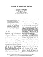
3. Acr length
A. Theoretical basis
➢ We can subdivide this curve into an infinite number of “near-straight” segments Δl
and sum them together. Consider 𝑥0 ∈ [𝑎; 𝑏] and Δx > 0 such that Δx∈ [𝑎; 𝑏]
➢ With Δx small enough, we consider the length
of the graph curve f(x) limiting between the
two lines x=𝑥0 and x=𝑥0 + Δx is the length of
the line connecting 2 points A and B as shown
in figure 3. And also because Δx is small, so
AB = (d) should be considered as the tangent
at x of f(x)
➢ So the arc length Δl ≈ AB =

Δx
𝑐𝑜𝑠𝑎

, with a is the

angle formed by the tangent AB at x of f(x)
and
the
axis

Ox,
so
tanα=f’(𝑥0 )
Therefore: Δl=Δx√𝒇’(𝒙𝟎 ) + 𝟏 (5)
B. Curve length in Cartesian coordinates
From (5) we take the sum of the lengths of the small “straight” segments together, we get the
(𝑆): 𝑦 = 𝑓(𝑥)
formula to calculate the curve length limited by {
is L
𝑥 = 𝑎 𝑎𝑛𝑑 𝑥 = 𝑏
Then:

𝒃

L= ∫𝒂 √[𝒇’(𝒙)]𝟐 + 𝟏 𝒅𝒙

Example 7: Calculate the length of the arc OA lying on
𝑥2

the parapol y= with a≠0, which O is the origin, A is a
2𝑎
point on the parabol whose latitude is t


t2

2𝑥

2a

2𝑎

We have: A(t, ) and y’(x) =

=

𝑥
𝑎

𝑡

𝑡

𝑥

Therefore L = ∫0 √[𝑦 ′ (𝑥)]2 + 1 𝑑𝑥 = ∫0 √( )2 + 1 𝑑𝑥
𝑎

1

= √𝑥 2 + 𝑎2 𝑑𝑥
𝑎
=
=

1
2𝑎

[x√𝑥 2 + 𝑎2 + 𝑎2 ln|𝑥 + √𝑥 2 + 𝑎2 |]| 0𝑡

𝑡

𝑎

√𝑡 2 + 𝑎2 +2 ln (
2𝑎

𝑡+√𝑡 2 +𝑎2
|𝑎|

)

C. Curve length with parametric equation
We demonstrate the complete analogy from how to convert the area of a plane figure in
Cartesian coordinates to the area of a plane bounded by a line with parametric equations (in
section 2)
𝑏

From then, instead of (5) we get: l = ∫𝑎 √[𝑥 ′ (𝑡)]2 + [𝑦 ′ (𝑡)]2 dx in 𝑅2
𝑏

= ∫𝑎 √[𝑥 ′ (𝑡)]2 + [𝑦 ′ (𝑡)]2 + [𝑧 ′ (𝑡)]2dx in 𝑅3
Example 8: Calculate the length of the arc of Archimedes’spiral
𝑥 = 𝑎𝑐𝑜𝑠𝑡
{𝑦 = 𝑎𝑠𝑖𝑛𝑡 𝑤𝑖𝑡ℎ 0 ≤ 𝑡 ≤ 2𝜋 𝑎𝑛𝑑 𝑎 > 0
𝑧 = 𝑎𝑡
We have: x’(t) = -asint, y’(t) = acost, z’(t) = a
2𝜋

Therefore L = ∫0 √[𝑥 ′ (𝑡)]2 + [𝑦 ′ (𝑡)]2 + [𝑧 ′ (𝑡)]2 𝑑𝑡

2𝜋

= ∫0 √(−𝑎𝑠𝑖𝑛𝑡)2 + (𝑎𝑐𝑜𝑠𝑡)2 + 𝑎2 𝑑𝑡
2𝜋

= a∫0 √𝑠𝑖𝑛𝑡 2 + 𝑐𝑜𝑠𝑡 2 + 1𝑑𝑡
2𝜋

= a√2 ∫0 𝑑𝑡 = a√2 | 2𝜋
= 2𝜋a√2
0

II.

ALGEBRAIC APPLICATIONS OF DEFINITE INTEGRAL
1. Integral inequality
We evalute the inequality in terms of functions and integrals


Example11: Prove that:
Consider f(x) =

1

𝜋
2

𝜋

< ∫0

16

1

𝑑𝑥 <

5 +3(𝑐𝑜𝑠𝑥)3

𝜋
10

𝜋

5 +3(𝑐𝑜𝑠𝑥)3

is continuous on [0; ]
2

𝜋

We have 0 ≤ cosx ≤ 1, for all x ϵ [0; ]
2
𝜋

Then: 0 ≤ (𝑐𝑜𝑠𝑥)3 ≤ 1, for all x ϵ [0; ]
1

1

=> ≤


2
𝜋

1

≤ , for all x ϵ [0; ]

5 +3(𝑐𝑜𝑠𝑥)3
5
𝜋
𝜋
1
1
= ∫02 𝑑𝑥 < ∫02
𝑑𝑥
16
8
5 +3(𝑐𝑜𝑠𝑥)3
8
𝜋

2

𝜋
1
2

< ∫0 𝑑𝑥 =
5

𝜋
10

2. Integral applications prove the inequality
Example 12: Prove that: ln(1+a) >

2𝑎
1+𝑎

, for all a > 1

1

+) In the coordinate system Oxy, consider the graph of the function (C): y = and set
𝑥0 =

𝑥

1+𝑎

ϵ [1;a]

2

1

Let the points A, B, C, D be A(1; 0), B(1+a; 0), C(𝑥0 ; 0), D(𝑥0 ; )

𝑥0

We have: y’ =

−1
𝑥2

=> y’’ =

−(−2𝑥)
(𝑥 2 )2

=

2

> 0, for all x > 0

𝑥3

1

Then: y = is a concave function, for all x > 0
𝑥
Two lines x = 1, x = 1+a intersect the tangent (d)
1
at D(𝑥0 ; ) at two points E, F and
𝑥0

1

intersect the graph (C): y =
1+𝑎 1

Then:𝑆𝐴𝐵𝐺𝐻 = ∫1

𝑥

𝑥

at two points H, G.

𝑑𝑥 = ln (1 + 𝑎)

+) We have: CD = √(𝑥0 − 𝑥0 )2 + (
But 𝑥0 =

1+𝑎
2

=> CD =

Therefore, 𝑆𝐴𝐵𝐺𝐻 = 𝐴𝐵.

1
1+𝑎
2

=

1
𝑥0

− 0)2 =

1
𝑥0

2

1+𝑎
𝐴𝐹+𝐵𝐸
2

(6)

= 𝐴𝐵. 𝐶𝐷 = 𝑎.

2
1+𝑎

=

2𝑎
1+𝑎

From (6) and (7) with 𝑆𝐴𝐵𝐺𝐻 > 𝑆𝐴𝐵𝐸𝐹 , we have ln(1+a) >

(7)
2𝑎

1+𝑎

, for all a > 1


Conclusion
Essay content"Integral Applications”Including methods of calculating primitives,
definite integrals and some applications of definite integrals, the essay has achieved some
important results:
+ The essay has demarcated and presented the method of calculating the area of a plane
figure, the length arc in geometrical applications of integrals. From there, apply
integration to practical problems and solve some common problems such as proving
inequality.
+ Is aimed at raising the reader's awareness of the integral and its application in
mathematics
Through the above analysis, we will have an overview and a more positive view of
integrals, about applications that are very close to reality. But in any field, two methods
total integral and differential diagram are always two directions for easy access and use
in practical problems. Today, calculus - integration requires learners and researchers to
have a deep understanding of the nature so that they can come up with new and more
practical applications, not just stopping at things that the group has already learned. tell.
In the process of implementation, the team has tried to limit errors but still cannot
avoid mistakes, so the essay is still incomplete and profound. The student group hopes to
receive more comments from readers.
Finally, the group would like to express their sincere thanks to Mr. Nguyen Van Thin's
support during the process of writing the essay.