COMPUTATIONAL MATERIALS ENGINEERINGAn Introduction to Microstructure Evolution.This page doc

COMPUTATIONAL
MATERIALS ENGINEERING
An Introduction to Microstructure Evolution
This page intentionally left blank
COMPUTATIONAL
MATERIALS ENGINEERING
An Introduction to Microstructure Evolution
KOENRAAD G. F. JANSSENS
DIERK RAABE
ERNST KOZESCHNIK
MARK A. MIODOWNIK
BRITTA NESTLER
AMSTERDAM
•
BOSTON
•
HEIDELBERG
•
LONDON
NEW YORK
•
OXFORD
•
PARIS
•
SAN DIEGO
SAN FRANCISCO
•
SINGAPORE
•

SYDNEY
•
TOKYO
Academic Press is an imprint of Elsevier
Elsevier Academic Press
30 Corporate Drive, Suite 400, Burlington, MA 01803, USA
525 B Street, Suite 1900, San Diego, California 92101-4495, USA
84 Theobald’s Road, London WC1X 8RR, UK
This book is printed on acid-free paper.
∞
Copyright
c
 2007, Elsevier Inc. All rights reserved.
No part of this publication may be reproduced or transmitted in any form or by any means, electronic or
mechanical, including photocopy, recording, or any information storage and retrieval system, without permission
in writing from the publisher.
Permissions may be sought directly from Elsevier’s Science & Technology Rights Department in Oxford, UK:
phone: (+44) 1865 843830, fax: (+44) 1865 853333, E-mail: You may also
complete your request on-line via the Elsevier homepage () , by selecting “Customer Support”
and then “Obtaining Permissions.”
Library of Congress Cataloging-in-Publication Data
Computational materials engineering: an introduction to microstructure evolution/editors Koenraad G. F.
Janssens [et al.].
p. cm.
Includes bibliographical references and index.
ISBN-13: 978-0-12-369468-3 (alk. paper)
ISBN-10: 0-12-369468-X (alk. paper)
1. Crystals–Mathematical models. 2. Microstructure–Mathematical models. 3. Polycrystals–Mathematical
models. I. Janssens, Koenraad G. F., 1968-
TA418.9.C7C66 2007

548

.7–dc22
2007004697
British Library Cataloguing-in-Publication Data
A catalogue record for this book is available from the British Library
ISBN 13: 978-0-12-369468-3
ISBN 10: 0-12-369468-X
For all information on all Elsevier Academic Press publications
visit our Web site at www.books.elsevier.com
Printed in the United States of America
07080910111210987654321
to Su
This page intentionally left blank
Table of Contents
Preface xiii
1 Introduction 1
1.1 Microstructures Defined 1
1.2 Microstructure Evolution 2
1.3 Why Simulate Microstructure Evolution? 4
1.4 Further Reading 5
1.4.1 On Microstructures and Their Evolution from
a Noncomputational Point of View 5
1.4.2 On What Is Not Treated in This Book 6
2 Thermodynamic Basis of Phase Transformations 7
2.1 Reversible and Irreversible Thermodynamics 8
2.1.1 The First Law of Thermodynamics 8
2.1.2 The Gibbs Energy 11
2.1.3 Molar Quantities and the Chemical Potential 11
2.1.4 Entropy Production and the Second Law of

Thermodynamics 12
2.1.5 Driving Force for Internal Processes 15
2.1.6 Conditions for Thermodynamic Equilibrium 16
2.2 Solution Thermodynamics 18
2.2.1 Entropy of Mixing 19
2.2.2 The Ideal Solution 21
2.2.3 Regular Solutions 22
2.2.4 General Solutions in Multiphase Equilibrium 25
2.2.5 The Dilute Solution Limit—Henry’s and Raoult’s Law 27
2.2.6 The Chemical Driving Force 28
2.2.7 Influence of Curvature and Pressure 30
2.2.8 General Solutions and the CALPHAD Formalism 33
2.2.9 Practical Evaluation of Multicomponent Thermodynamic
Equilibrium 40
vii
3 Monte Carlo Potts Model 47
3.1 Introduction 47
3.2 Two-State Potts Model (Ising Model) 48
3.2.1 Hamiltonians 48
3.2.2 Dynamics (Probability Transition Functions) 49
3.2.3 Lattice Type 50
3.2.4 Boundary Conditions 51
3.2.5 The Vanilla Algorithm 53
3.2.6 Motion by Curvature 54
3.2.7 The Dynamics of Kinks and Ledges 57
3.2.8 Temperature 61
3.2.9 Boundary Anisotropy 62
3.2.10 Summary 64
3.3
Q-State Potts Model 64

3.3.1 Uniform Energies and Mobilities 65
3.3.2 Self-Ordering Behavior 67
3.3.3 Boundary Energy 68
3.3.4 Boundary Mobility 72
3.3.5 Pinning Systems 75
3.3.6 Stored Energy 77
3.3.7 Summary 80
3.4 Speed-Up Algorithms 80
3.4.1 The Boundary-Site Algorithm 81
3.4.2 The N-Fold Way Algorithm 82
3.4.3 Parallel Algorithm 84
3.4.4 Summary 87
3.5 Applications of the Potts Model 87
3.5.1 Grain Growth 87
3.5.2 Incorporating Realistic Textures and Misorientation
Distributions 89
3.5.3 Incorporating Realistic Energies and Mobilities 92
3.5.4 Validating the Energy and Mobility Implementations 93
3.5.5 Anisotropic Grain Growth 95
3.5.6 Abnormal Grain Growth 98
3.5.7 Recrystallization 102
3.5.8 Zener Pinning 103
3.6 Summary 107
3.7 Final Remarks 107
3.8 Acknowledgments 108
4 Cellular Automata 109
4.1 A Definition 109
4.2 A One-Dimensional Introduction 109
4.2.1 One-Dimensional Recrystallization 111
4.2.2 Before Moving to Higher Dimensions 111

4.3 +2D CA Modeling of Recrystallization 116
4.3.1 CA-Neighborhood Definitions in Two Dimensions 116
4.3.2 The Interface Discretization Problem 118
4.4 +2D CA Modeling of Grain Growth 123
viii TABLE OF CONTENTS
4.4.1 Approximating Curvature in a Cellular Automaton Grid 124
4.5 A Mathematical Formulation of Cellular Automata 128
4.6 Irregular and Shapeless Cellular Automata 129
4.6.1 Irregular Shapeless Cellular Automata for Grain Growth 131
4.6.2 In the Presence of Additional Driving Forces 135
4.7 Hybrid Cellular Automata Modeling 136
4.7.1 Principle 136
4.7.2 Case Example 137
4.8 Lattice Gas Cellular Automata 140
4.8.1 Principle—Boolean LGCA 140
4.8.2 Boolean LGCA—Example of Application 142
4.9 Network Cellular Automata—A Development for the Future? 144
4.9.1 Combined Network Cellular Automata 144
4.9.2 CNCA for Microstructure Evolution Modeling 145
4.10 Further Reading 147
5 Modeling Solid-State Diffusion 151
5.1 Diffusion Mechanisms in Crystalline Solids 151
5.2 Microscopic Diffusion 154
5.2.1 The Principle of Time Reversal 154
5.2.2 A Random Walk Treatment 155
5.2.3 Einstein’s Equation 157
5.3 Macroscopic Diffusion 160
5.3.1 Phenomenological Laws of Diffusion 160
5.3.2 Solutions to Fick’s Second Law 162
5.3.3 Diffusion Forces and Atomic Mobility 164

5.3.4 Interdiffusion and the Kirkendall Effect 168
5.3.5 Multicomponent Diffusion 171
5.4 Numerical Solution of the Diffusion Equation 174
6 Modeling Precipitation as a Sharp-Interface Phase Transformation 179
6.1 Statistical Theory of Phase Transformation 181
6.1.1 The Extended Volume Approach—KJMA Kinetics 181
6.2 Solid-State Nucleation 185
6.2.1 Introduction 185
6.2.2 Macroscopic Treatment of Nucleation—Classical Nucleation
Theory 186
6.2.3 Transient Nucleation 189
6.2.4 Multicomponent Nucleation 191
6.2.5 Treatment of Interfacial Energies 194
6.3 Diffusion-Controlled Precipitate Growth 197
6.3.1 Problem Definition 199
6.3.2 Zener’s Approach for Planar Interfaces 202
6.3.3 Quasi-static Approach for Spherical Precipitates 203
6.3.4 Moving Boundary Solution for Spherical Symmetry 205
6.4 Multiparticle Precipitation Kinetics 206
6.4.1 The Numerical Kampmann–Wagner Model 206
6.4.2 The SFFK Model—A Mean-Field Approach for Complex
Systems 209
6.5 Comparing the Growth Kinetics of Different Models 215
TABLE OF CONTENTS ix
7 Phase-Field Modeling 219
7.1 A Short Overview 220
7.2 Phase-Field Model for Pure Substances 222
7.2.1 Anisotropy Formulation 224
7.2.2 Material and Model Parameters 226
7.2.3 Application to Dendritic Growth 226

7.3 Case Study 228
7.3.1 Phase-Field Equation 229
7.3.2 Finite Difference Discretization 229
7.3.3 Boundary Values 231
7.3.4 Stability Condition 232
7.3.5 Structure of the Code 232
7.3.6 Main Computation 233
7.3.7 Parameter File 236
7.3.8 MatLab Visualization 237
7.3.9 Examples 238
7.4 Model for Multiple Components and Phases 241
7.4.1 Model Formulation 241
7.4.2 Entropy Density Contributions 242
7.4.3 Evolution Equations 245
7.4.4 Nondimensionalization 248
7.4.5 Finite Difference Discretization and Staggered Grid 249
7.4.6 Optimization of the Computational Algorithm 252
7.4.7 Parallelization 253
7.4.8 Adaptive Finite Element Method 253
7.4.9 Simulations of Phase Transitions and Microstructure
Evolution 253
7.5 Acknowledgments 265
8 Introduction to Discrete Dislocations Statics and Dynamics 267
8.1 Basics of Discrete Plasticity Models 267
8.2 Linear Elasticity Theory for Plasticity 268
8.2.1 Introduction 268
8.2.2 Fundamentals of Elasticity Theory 269
8.2.3 Equilibrium Equations 273
8.2.4 Compatibility Equations 274
8.2.5 Hooke’s Law—The Linear Relationship between Stress and

Strain 275
8.2.6 Elastic Energy 280
8.2.7 Green’s Tensor Function in Elasticity Theory 280
8.2.8 The Airy Stress Function in Elasticity Theory 283
8.3 Dislocation Statics 284
8.3.1 Introduction 284
8.3.2 Two-Dimensional Field Equations for Infinite Dislocations
in an Isotropic Linear Elastic Medium 285
8.3.3 Two-Dimensional Field Equations for Infinite Dislocations
in an Anisotropic Linear Elastic Medium 287
8.3.4 Three-Dimensional Field Equations for Dislocation Segments
in an Isotropic Linear Elastic Medium 289
x TABLE OF CONTENTS
8.3.5 Three-Dimensional Field Equations for Dislocation Segments
in an Anisotropic Linear Elastic Medium 292
8.4 Dislocation Dynamics 298
8.4.1 Introduction 298
8.4.2 Newtonian Dislocation Dynamics 299
8.4.3 Viscous and Viscoplastic Dislocation Dynamics 307
8.5 Kinematics of Discrete Dislocation Dynamics 310
8.6 Dislocation Reactions and Annihilation 311
9 Finite Elements for Microstructure Evolution 317
9.1 Fundamentals of Differential Equations 317
9.1.1 Introduction to Differential Equations 317
9.1.2 Solution of Partial Differential Equations 320
9.2 Introduction to the Finite Element Method 321
9.3 Finite Element Methods at the Meso- and Macroscale 322
9.3.1 Introduction and Fundamentals 322
9.3.2 The Equilibrium Equation in FE Simulations 324
9.3.3 Finite Elements and Shape Functions 324

9.3.4 Assemblage of the Stiffness Matrix 327
9.3.5 Solid-State Kinematics for Mechanical Problems 329
9.3.6 Conjugate Stress–Strain Measures 331
Index 335
TABLE OF CONTENTS xi
This page intentionally left blank
Preface
Being actively involved since 1991 in different research projects that belong under the field of
computational materials science, I always wondered why there is no book on the market which
introduces the topic to the beginning student. In 2005 I was approached by Joel Stein to write
a book on this topic, and I took the opportunity to attempt to do so myself. It was immediately
clear to me that such a task transcends a mere copy and paste operation, as writing for experts is
not the same as writing for the novice. Therefore I decided to invite a respectable collection of
renowned researchers to join me on the endeavor. Given the specific nature of my own research,
I chose to focus the topic on different aspects of computational microstructure evolution. This
book is the result of five extremely busy and active researchers taking a substantial amount of
their (free) time to put their expertise down in an understandable, self-explaining manner. I am
very grateful for their efforts, and hope the reader will profit. Even if my original goals were
not completely met (atomistic methods are missing and there was not enough time do things as
perfectly as I desired), I am satisfied with—and a bit proud of—the result.
Most chapters in this book can be pretty much considered as stand-alones. Chapters 1 and 2
are included for those who are at the very beginning of an education in materials science; the
others can be read in any order you like.
Finally, I consider this book a work in progress. Any questions, comments, corrections, and
ideas for future and extended editions are welcome at You may also
want to visit the web site accompanying this book at http:// books.elsevier.com/companions/
9780123694683.
Koen Janssens,
Linn, Switzerland,
December 2006

xiii
This page intentionally left blank
1 Introduction
—Koen Janssens
The book in front of you is an introduction to computational microstructure evolution. It is not
an introduction to microstructure evolution. It does assume you have been sufficiently intro-
duced to materials science and engineering to know what microstructure evolution is about.
That being said we could end our introduction here and skip straight to the computational
chapters. However, if you intend to learn more about the science of polycrystalline materials but
want to learn about them through their computational modeling, then this chapter will give you
the bare-bones introduction to the secrets of microstructures. Just remember that the one law
binding any type of computational modeling is equally valid for computational microstructure
evolution:
garbage-in
= garbage-out (1.1)
You have been warned—we wash our hands in innocence.
1.1 Microstructures Defined
The world of materials around us is amazingly diverse. It is so diverse that scientists feel the need
to classify materials into different types. Like the authors of this book, your typical technologist
classifies materials based on their technical properties. Fundamental groups are, for example,
metals and alloys, ceramics, polymers, and biomaterials. More specific classifications can be,
for example, semiconductors, nanomaterials, memory alloys, building materials, or geologic
minerals.
In this book the focus is on materials with polycrystalline microstructures. For the sake of
simplicity let us consider a pure metal and start with atoms as the basic building blocks. The
atoms in a metal organize themselves on a crystal lattice structure. There are different types
of lattice structures each with their defining symmetry. Auguste Bravais was the first to classify
them correctly in 1845, a classification published in 1850–1851 [Bra, Bra50, Bra51]. The lattice
parameters define the length in space over which the lattice repeats itself, or in other words the
volume of the unit cell of the crystal. The organization of atoms on a lattice with a specific set of

lattice parameters is what we call a solid state phase. Going from pure metals to alloys, ceram-
ics, polymers, and biomaterials, the structures get more and more complex and now consist
of lattices of groups of different atoms organized on one or more different lattice structures.
1
For completeness it should be mentioned that not in all materials are the atoms organized
on lattices; usually the larger the atom groups the less it becomes probable—like for most
polymers—and we end up with amorph or glassy structures in the material.
The most simple microstructure is a perfect single crystal. In a perfect single crystal the
atoms are organized on a crystal lattice without a single defect. What crystal structure the atoms
organize on follows from their electronic structure. Ab initio atomistic modeling is a branch of
computational materials science concerning itself with the computation of equilibrium crystal
structures. Unfortunately we do not treat any form of molecular dynamics in this book—or, to
be more honest would be to admit we did not make the deadline. But keep your wits up, we are
considering it for a future version of this book, and in the meantime refer to other publications
on this subject (see Section 1.4 at the end of this chapter).
When the material is not pure but has a composition of elements
1
, the lattice is also modified
by solute or interstitial atoms that are foreign to its matrix. Depending on temperature and
composition, a material may also have different phases, meaning that the same atoms can be
arranged in different crystal lattice structures, the equilibrium phase being that one which has
the lowest Gibbs free energy at a particular temperature and pressure. If you lost me when
I used the words “Gibbs free energy” you may want to read Chapter 2 in this book (and needless
to say, if you are an expert on the matter you may wish to skip that chapter, unless of course
you feel like sending us some ideas and corrections on how to make this book a better one).
In any case, but especially in view of equation (1.1), it is important that you have a minimum
of understanding of materials thermodynamics.
Any deviation from a material’s perfect single-crystal structure increases the energy stored in
the material by the introduction of crystal defects. These defects are typically classified accord-
ing to their dimensions in space: point defects, line defects, and surface defects. Important in

the context of microstructures is that the energy stored in these defects is a driving force for
microstructure transformation. For example, a grain boundary is a defect structure, and the
microstructure is thereby driven to minimize its free energy by minimizing the surface area of
grain boundaries in itself, hence the process of grain growth. In a deformed microstructure of a
metal, the dislocations can be removed from the microstructure by recovery, in which disloca-
tions mutually annihilate, but also by the nucleation and growth of new, relatively dislocation-
free grains, hence the process of recrystallization. Phase transformations are similar in that they
also involve nucleation and growth of grains, but are different in the origin of the driving force,
which is now the difference of the free energy density of different phases of the same crystal.
Once again, you can read more about all the underlying thermodynamics in Chapter 2. Another
point to keep in mind is that other properties, such as grain boundary mobility, may be coupled
to the presence of defects in a crystal.
At this point we have defined most of the relevant concepts and come back to what the
microstructure of a polycrystalline material is:
A microstructure is a spatially connected collection of arbitrarily shaped grains separated by grain
boundaries, where each grain is a (possibly-non-defect-free) single crystal and the grain boundaries
are the location of the interfaces between grains.
1.2 Microstructure Evolution
Now that you have some idea of what microstructures are, we can start talking about
microstructure evolution. Evolution is actually an unfortunate word choice, as microstructures
1
A real material is always composed of a multitude of elements, leading to the saying that “materials science is
the physics of dirt” [Cah02]—but that is another story
2 COMPUTATIONAL MATERIALS ENGINEERING
do not evolve in the way living materials do. The use of the word evolution probably originated
from an attempt to find generalized wording for the different transformation processes that
are observed in changing microstructures. The word “transformation” is somewhat reserved
to “phase transformation” when speaking about microstructures. A better term possibly would
have been microstructure transmutation, as it points more precisely at what is really meant:
under the influence of external heat and/or work, a microstructure transmutes into another

microstructure.
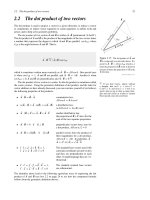
But let us keep it simple and explain what microstructure evolution is by illustration with an
example from the metal processing industry shown in Figure 1-1. The figure shows how a metal
is continuously cast and subsequently hot rolled. Many different microstructure transformations
come into action in this complex materials processing line:
Solidification: Solidification is the process which defines the casting process at the microstruc-
ture scale. Solidification is a phase transformation, special because a liquid phase
transforms into a solid phase. In this book you can find examples of the simulation of
solidification using the phase-field method in Chapter 7.
Diffusion: Diffusion also is one of the main characters, for example, in the segregation of
elements in front of the solidification front. But diffusion is a process which plays a
role in any microstructure transformation at an elevated temperature, be it the anneal-
ing after casting or before and during hot rolling (or any other technological process
Gibbs energy of mixing ∆GTemperature T
T
2
<<T
cr
T
2
<T
cr
T
4
>T
cr
T
5
>>T
cr

T
3
= T
cr
T
cr
T
2
T
1
0 0.2 0.6 0.8 10.4
G
1,unstable
G
1,equilibrium
Phase Transformation
Diffusion
Solidification
Grain Growth
Deformation
Recrystallization
Recovery
Molefraction X
B
FIGURE 1-1 Schematic of the industrial processing of a metal from its liquid phase to a sheet metal,
showing the different microstructure transformations which occur.
Introduction 3
involving heat treatments). You can find information on the modeling of the diffusion
process in Chapter 5.
Phase Transformation: Phase transformation is microstructural transformation in the solid

state that occurs at elevated temperature heat treatments when a material has different
thermodynamically stable phases at different temperatures, like iron has an face centered
cubic phase (austenite) and a body centered cubic phase (ferrite). Phase transformations
can be modeled computationally using a variety of methods, several of which are intro-
duced in this book. The phase-field model is treated in Chapter 7, and although not explic-
itly treated, Potts-type Monte Carlo in Chapter 3 and cellular automata in Chapter 4 are a
possibility. Read more about the underlying thermodynamics in Chapter 6.
Deformation: The plastic deformation of a metal is a topic that has been studied since the
beginning of materials science. Plasticity can be modeled at the continuum scale, and
recently the field of multiscale modeling is slowly but certainly closing the gap between
the microstructure and the continuum scales of computational modeling. In this book we
only touch on plasticity with the description of two computational approaches. Closer
to the atomistic scale is discrete dislocation dynamics modeling, which is introduced in
Chapter 8. Coming from the scale of continuum modeling, we also treat the application
of finite elements to microstructure evolution modeling in Chapter 9. The recovery of a
plastically deformed metal is in essence a process at the dislocation scale, but it is not
addressed in this book.
Recrystallization and Grain Growth: Recrystallization and grain growth, on the other hand,
are treated in detail as an application of cellular automata in Chapter 4 and of Potts-type
Monte Carlo in Chapter 3.
1.3 Why Simulate Microstructure Evolution?
Modern materials are characterized by a wide spectrum of tailored mechanical, optical, mag-
netic, electronic, or thermophysical properties. Frequently these properties can be attributed to
a specially designed microstructure.
A dedicated microstructure of a metal promoting its strength and toughness could be one
with small and homogeneous grains, minimum impurity segregation, and a high number density
of small, nanometer-sized precipitates to stabilize grain boundaries and dislocations. To obtain
this particular microstructure in the course of the material manufacturing processes, advantage
is oft taken of different microstructural transformation processes that have the power of pro-
ducing the desired microstructures in a reproducible way, such as depicted in Figure 1-1: phase

transformation, diffusion, deformation, recrystallization, and grain growth.
Today, computational modeling is one of the tools at the disposal of scientific engineers,
helping them to better understand the influence of different process parameters on the details
of the microstructure. In some cases such computational modeling can be useful in the opti-
mization of the microstructure to obtain very specific material properties, and in specific cases
modeling may be used directly to design new microstructures. In spite of the fact that the latter is
frequently used as an argument in favor of computational materials science, the true strength of
the computational approach is still its use as a tool for better understanding. Technologically rel-
evant microstructures are four-dimensional (in space and time ) creatures that are difficult for the
human mind to grasp correctly. That this understanding is relevant becomes obvious when one
reads the way Martin, Doherty, and Cantor view microstructures [MDC97]: a microstructure
is a meta-stable structure that is kinetically prevented to evolve into a minimum free-energy
4 COMPUTATIONAL MATERIALS ENGINEERING
configuration. This means that to produce a specific microstructure, one must understand the
kinetic path along which it evolves, and be able to stop its evolution at the right moment in
processing time.
With the help of computational modeling, the scientist is able to dissect the microstructure in
space and in its evolution in time, and can, for example, perform different parameter studies to
decide how to ameliorate the manufacturing process. Building such a computational tool always
needs three components:
1. Having correct models defining the underlying physics of the different subprocesses that
act in the play of microstructure evolution, for example, diffusion equations or laws for
grain boundary migration or dislocation motion.
2. A computational model, which is capable of simulating the evolution of the microstruc-
ture using the underlying laws of physics as input. A major concern in such a model is
always that the different sub-models compute on the same scale. As an example, it is
relatively straightforward to model recovery of a deformed metal analytically, fitting the
parameters to experimental data. It is already much more complex to model recrystal-
lization using cellular automata, as it is not so straightforward to calibrate the length of
an incremental step in the model against real time. The latter is usually circumvented

by normalizing the simulation and experimental data based on particular points in time
(e.g., a certain amount of the volume recrystallized), but such assumes that the relation
between time and simulation step is linear, which is not always true. Combining both the
analytical recovery model and the computational recrystallization model requires a true
time calibration so this trick can no longer be applied, resulting in tedious time calibra-
tion experiments and simulations that need be performed with great care if one aims to
transcend mere qualitative predictions.
3. Finally, unless one is studying the microstructure itself, one needs additional modeling,
which relates the (simulated) microstructures on the one side, to the target properties on
the other side of the equation. Such a model would, for example, compute the plastic
yield locus of a metal based on characteristics of the microstructure such as the grain size
distribution. It should need little imagination to realize that such a computation can easily
be equally complex as the microstructure evolution model itself.
This book focuses entirely on item 2 in the preceding list. For the less sexy topics the reader is
referred to other monographs—see further reading.
1.4 Further Reading
1.4.1 On Microstructures and Their Evolution from a Noncomputational
Point of View
The book by Humphreys and Hatherly [HH96] is certainly one of the most referenced books
on this topic and gives a good overview. Other important monographs I would consider are
the work of Gottstein and Shvindlerman [GS99] on the physics of grain boundary migration in
metals, the book of Martin, Doherty, and Cantor [MDC97] on the stability of microstructures,
and Sutton and Balluffi [SB95] on interfaces in crystalline materials. Finally, if you need decent
mathematics to compute crystal orientations and misorientations, Morawiec’s work [Mor04]
may help.
Introduction 5
1.4.2 On What Is Not Treated in This Book
Unfortunately we did not have time nor space to treat all methods you can use for microstructure
evolution modeling. If you did not find your taste in our book, here are some other books we
prudently suggest.

Molecular Dynamics: Plenty of references here. Why not start with a classic like Frenkel and
Smit [FS96]?
Level Set: Level set methods and fast marching methods are in the book of Sethian [Set99].
Continuum Plasticity of Metals: Yes, continuum theory also finds its application in the sim-
ulation of microstructures, especially when it concerns their deformation. Actually, you
can find its application to microstructure evolution in this book in Chapter 9. Other mono-
graphs on the subject in general are plenty. Lemaitre and Chaboche [LC90] certainly gives
a very good overview, but it may be on the heavy side for the beginning modeler. An eas-
ier point of entry may be Han and Reddy [HR99] on the mathematics of plasticity, and
Dunne and Petrinic [DP05] on its computational modeling.
Particle Methods: See Liu and Liu [LL03].
Genetic Algorithms: Because you never know when you may need these, the book by Haupt
and Haupt [HH04] describes the basic ideas really well.
The Meshless Local Petrov-Galerkin (MLPG) Method, S. N. Atluri and S. Shen, Tech Science
Press, Forsyth, GA, 2002. [Atl02]
See Torquato [Tor02] on methods for computational modeling of the relation between
microstructure and materials properties!
Bibliography
[Bra] M. A. Bravais. />–
lattice.
[Bra50] M. A. Bravais. J. Ecole Polytechnique, 19:1–128, 1850.
[Bra51] M. A. Bravais. J. Ecole Polytechnique, 20:101–278, 1851.
[Cah02] R. W. Cahn. The science of dirt. Nature Materials, 1:3–4, 2002.
[DP05] F. Dunne and N. Petrinic. Introduction to Computational Plasticity. Oxford University Press, Oxford, 2005.
[FS96] D. Frenkel and B. Smit. Understanding Molecular Simulation. Academic Press, San Diego, 1996.
[GS99] G. Gottstein and L. S. Shvindlerman. Grain Boundary Migration in Metals. CRC Press LLC, Boca Raton,
FL, 1999.
[HH96] F. J. Humphreys and M. Hatherly. Recrystallization and Related Annealing Phenomena. Pergamon,
Oxford, 1996.
[HH04] R. L. Haupt and S. E. Haupt. Practical Genetic Algorithms. Wiley, Hoboken, NJ, 2004.

[HR99] W. Han and B. D. Reddy. Plasticity—Mathematical Theory and Numerical Analysis. Springer-Verlag,
Berlin, 1999.
[LC90] J. Lemaitre and J L. Chaboche. Mechanics of Solid Materials. Cambridge University Press, Cambridge,
1990.
[LL03] G. R. Liu and M. B. Liu. Smoothed Particle Hydrodynamics. World Scientific, London, 2003.
[MDC97] J. W. Martin, R. D. Doherty, and B. Cantor. Stability of Microstructures in Metallic Systems. Cambridge
University Press, Cambridge, 1997.
[Mor04] A. Morawiec. Orientations and Rotations: Computations in Crystallographic Textures. Springer-Verlag,
Berlin, 2004.
[SB95] A. P. Sutton and R. W. Balluffi. Interfaces in Crystalline Materials. Clarendon Press, Oxford, 1995.
[Set99] J. A. Sethian. Level Set Methods and Fast Marching Methods. Cambridge University Press, Cambridge,
1999.
[Tor02] S. Torquato. Random Heterogeneous Materials: Microstructure and Macroscopic Properties. Springer-
Verlag, Berlin, 2002.
[Atl02] S. N. Atluri and S. Shen. The Meshless Local Petrov-Galerkin (MLPG) Method. Tech Science Press,
Forsyth, GA, 2002.
6 COMPUTATIONAL MATERIALS ENGINEERING
2 Thermodynamic Basis of Phase
Transformations
—Ernst Kozeschnik
Many of the models that are discussed in this book rely on the knowledge of thermodynamic
quantities, such as solution enthalpies, chemical potentials, driving forces, equilibrium mole
fractions of components, etc. These quantities are needed as model input parameters and they are
often not readily available in experimental form when dealing with special or complex systems.
However, in the last decades, suitable theoretical models have been developed to assess and
collect thermodynamic and kinetic data and store them in the form of standardized databases.
Thus, essential input data for modeling and simulation of microstructure evolution is accessible
on the computer.
Although thermodynamics is covered in numerous excellent textbooks and scientific publi-
cations, we nevertheless feel the strong necessity to introduce the reader to the basic concepts

of thermodynamics, and in particular to solution thermodynamics (Section 2.2), which we will
be most concerned with in computational modeling of microstructure evolution. The basics are
discussed at least to a depth that the theoretical concepts of the modeling approaches can be
understood and correctly applied and interpreted as needed in the context of this book. Some of
the material that is presented subsequently is aimed at giving the reader sufficient understanding
of the underlying approaches to apply theory in the appropriate way. Some of it is aimed at
providing reference material for later use.
Thermodynamics provides a very powerful methodology for describing macroscopic observ-
ables of materials on a quantitative basis. In the last decades, mathematical and computational
methods have been developed to allow extrapolation of known thermodynamic properties of
binary and ternary alloys into frequently unexplored higher-order systems of technical rele-
vance. The so-called method of computational thermodynamics (CT) is an indispensable tool
nowadays in development of new materials, and it has found its way into industrial practice
where CT assists engineers in optimizing heat treatment procedures and alloy compositions.
Due to the increasing industrial interest, comprehensive thermodynamic databases are being
developed in the framework of the CALPHAD (CALculation of PHAse Diagrams) technique,
which in combination with commercial software for Gibbs energy minimization can be used to
predict phase stabilities in almost all alloy systems of technical relevance [KEH
+
00]. More and
more students become acquainted with commercial thermodynamic software packages such
7
as ThermoCalc [SJA85], MTData [DDC
+
89], F*A*C*T [PTBE89], ChemSage [EH90], or
PANDAT [CZD
+
03] already at universities, where CT is increasingly taught as an obligatory
part of the curriculum.
Traditionally, computational thermodynamics is connected to the construction of phase dia-

grams on the scientist’s and engineer’s desktop. There, it can provide information about which
stable phases one will find in a material in thermodynamic equilibrium at a given temperature,
pressure, and overall chemical composition. This knowledge is already of considerable value to
the engineer when trying to identify, for instance, solution temperatures of wanted and unwanted
phases to optimize industrial heat treatments. Moreover, and this is of immediate relevance for
the present textbook: although the thermodynamic parameters that are stored in the thermody-
namic databases have been assessed to describe equilibrium conditions, these data also provide
information on thermodynamic quantities in the nonequilibrium state. For instance, chemical
potentials of each element in each phase can be evaluated for given temperature, pressure, and
phase composition. From these data, the chemical driving forces can be derived and finally used
in models describing kinetic processes such as phase transformations or precipitate nucleation
and growth.
It is not the intent of the present book to recapitulate solution thermodynamics in scientific
depth, and we will restrict ourselves to an outline of the basic concepts and methods in order
to provide the reader with the necessary skills to apply these theories in appropriate ways. For
a more comprehensive treatment, the reader is refered to some of the many excellent textbooks
on solution thermodynamics (e.g., refs. [Hil98, SM98, Cal85, Hac96, MA96, Wag52, FR76]) .
2.1 Reversible and Irreversible Thermodynamics
2.1.1 The First Law of Thermodynamics
Thermodynamics is a macroscopic art dealing with energy and the way how different forms of
energy can be transformed into each other. One of the most fundamental statements of thermo-
dynamics is related to the conservation of energy in a closed system, that is, a system with a
constant amount of matter and no interactions of any kind with the surrounding. When intro-
ducing the internal energy
U as the sum of all kinetic, potential, and interaction energies in the
system, we can define
U formally as a part Q coming from the heat that has flown into the
system and a part
W coming from the work done on the system:
U = Q + W (2.1)

It is important to recognize that this definition does not provide information about the abso-
lute value of
U and, in this form, we are always concerned with the problem of defining an
appropriate reference state. Therefore, instead of using the absolute value of the internal energy,
it is often more convenient to consider the change of
U during the transition from one state to
another and to use equation (2.1) in its differential form as
dU =dQ +dW (2.2)
By definition, the internal energy
U of a closed system is constant. Therefore, equation (2.2)
tells us that, in systems with constant amount of matter and in the absence of interactions with
the surrounding, energy can neither be created nor destroyed, although it can be converted from
one form into another. This is called the first law of thermodynamics.
8 COMPUTATIONAL MATERIALS ENGINEERING
The internal energy U is a state function because it is uniquely determined for each
combination of the state variables temperature
T , pressure P , volume V, and chemical compo-
sition
N. The vector N contains the numbers N
i
of moles of components i. Any thermodynamic
property that is independent of the size of the system is called an intensive property. Examples
for intensive quantities are
T and P or the chemical potential µ. An intensive state variable
or function is also denoted as a thermodynamic potential. A property that depends on the size
of the system is called an extensive property. Typical examples are the state variable
V or the
state function
U.
The value of a state function is always independent of the way how a certain state has been

reached, and for the internal energy of a closed system we can write

dU =0
(2.3)
A necessary prerequisite for the validity of equation (2.3) is that the variation of the state
variables is performed in infinitesimally small steps, and the process thus moves through a
continuous series of equilibria. In other words, after variation of any of the state variables,
we are allowed to measure any thermodynamic quantity only after the system has come to a
complete rest.
It is also important to realize that the state variables introduced before are not independent
of each other: If we have
c independent components in the system, only c +2state variables
can be chosen independently. For instance, in an ideal one-component gas (
c =1), we have the
four state variables
P , T , V , and N. Any three of these variables can be chosen independently,
while the fourth parameter is determined by the ideal gas law
PV = NRT. R is the universal
gas constant (
R =8.3145 J(mol K)
−1
). The choice of appropriate state variables is dependent
on the problem one is confronted with. In solution thermodynamics, a natural choice for the set
of state variables is
T , P , and N.
The quantities
Q and W are not state functions because the differentials dQ and dW simply
describe the interaction of the system with its surrounding or the interaction between two sub-
systems that are brought into contact. Depending on the possibilities of how a system can
exchange thermal and mechanical energy with its surrounding, different expressions for

dQ
and dW will be substituted into equation (2.2). For instance, a common and most important
path for mechanical interaction of two systems is the work done against hydrostatical pressure.
For convenience, a new function
H is introduced first with
H = U + PV (2.4)
which is called enthalpy.
H is also a state function and in its differential form we have
dH =dU + P dV + V dP (2.5)
Now consider an insulated cylinder filled with ideal gas and a frictionless piston on one
side. If the temperature of the gas is increased by an infinitesimal amount
dT and the pressure
of the gas is held constant, the piston must move outwards because the volume of the gas has
increased by the infinitesimal amount
dV . In the course of this process, work dW is done against
the hydrostatic pressure
P and we have
dW = −PdV (2.6)
Thermodynamic Basis of Phase Transformations 9
The minus sign comes from the fact that dW is defined as the mechanical energy received
by the system. Substituting equations (2.2) and (2.6) into the general definition (2.5) leads to
dH =dQ + V dP (2.7)
Under constant pressure and constant chemical composition (
dP =0, dN
i
=0), equation (2.7)
reduces to
(dH)
P,N
=dQ (2.8)

thus manifesting that the addition of any amount of heat
dQ to the system under these conditions
is equal to the increase
dH. If we further assume a proportionality between dH and dT ,we
can write
(dH)
P,N
= C
P
· dT (2.9)
The proportionality constant
C
P
is called specific heat capacity, and it is commonly inter-
preted as the amount of heat that is necessary to increase the temperature of one mole of atoms
by one degree. Formally, the definition of the specific heat capacity is written
C
P
=

∂H
∂T

P,N
(2.10)
The enthalpy
H has been introduced for conditions of constant pressure, constant chemical
composition, and under the assumption that
dW in equation (2.2) is representing a work done
against a hydrostatic pressure. An analogy will now be sought for the incremental heat

dQ.
In the previous example we have expressed the mechanical work input as
−∆W =∆(PV)
and used the differential form with
−dW = PdV + V dP (2.11)
In analogy to the mechanical part, we assume that the stored heat in the system can be
expressed by a product
∆Q =∆(TS). For the differential form we can write
dQ = T dS + SdT (2.12)
If heat is added under conditions of constant temperature, we finally arrive at the so-called
thermodynamic definition of entropy:
dS =
dQ
T
(2.13)
The concept of entropy was introduced by the German physicist Rudolf Clausius
(1822–1888). The word entropy has Greek origin and means transformation. Similar to
U
and H, entropy S is a state function. Its value is only dependent on the state variables T ,
P , V , N and it is independent of the way how the state was established. We can therefore
also write

dS =

dQ
T
=0
(2.14)
10 COMPUTATIONAL MATERIALS ENGINEERING