Đề tài " Approximating a bandlimited function using very coarsely quantized data: A family of stable sigma-delta modulators of arbitrary order " pptx
Bạn đang xem bản rút gọn của tài liệu. Xem và tải ngay bản đầy đủ của tài liệu tại đây (929.98 KB, 33 trang )
Annals of Mathematics
Approximating a bandlimited function
using very coarsely quantized data:
A family of stable sigma-delta
modulators of arbitrary order
By Ingrid Daubechies and Ron DeVore
Annals of Mathematics, 158 (2003), 679–710
Approximating a bandlimited function
using very coarsely quantized data:
A family of stable sigma-delta
modulators of arbitrary order
By Ingrid Daubechies and Ron DeVore
1. Introduction
Digital signal processing has revolutionized the storage and transmission
of audio and video signals as well as still images, in consumer electronics
and in more scientific settings (such as medical imaging). The main ad-
vantage of digital signal processing is its robustness: although all the oper-
ations have to be implemented with, of necessity, not quite ideal hardware, the
a priori knowledge that all correct outcomes must lie in a very restricted set
of well-separated numbers makes it possible to recover them by rounding off
appropriately. Bursty errors can compromise this scenario (as is the case in
many communication channels, as well as in memory storage devices), making
the “perfect” data unrecoverable by rounding off. In this case, knowledge of
the type of expected contamination can be used to protect the data, prior to
transmission or storage, by encoding them with error correcting codes; this is
done entirely in the digital domain. These advantages have contributed to the
present widespread use of digital signal processing.
Many signals, however, are not digital but analog in nature; audio signals,
for instance, correspond to functions f(t), modeling rapid pressure oscillations,
which depend on the “continuous” time t (i.e. t ranges over
or an interval
in
, and not over a discrete set), and the range of f typically also fills an
interval in
.For this reason, the first step in any digital processing of such
signals must consist in a conversion of the analog signal to the digital world,
usually abbreviated as A/D conversion. For different types of signals, different
A/D schemes are used; in this paper, we restrict our attention to a particular
class of A/D conversion schemes adapted to audio signals. Note that at the end
of the chain, after the signal has been processed, stored, retrieved, transmitted,
, all in digital form, it needs to be reconverted to an analog signal that can
be understood by a human hearing system; we thus need a D/A conversion
there.
680 INGRID DAUBECHIES AND RON DEVORE
The digitization of an audio signal rests on two pillars: sampling and
quantization,both of which we now briefly discuss.
We start with sampling. It is standard to model audio signals by band-
limited functions, i.e. functions f ∈ L
2
( ) for which the Fourier transform
ˆ
f(ξ)=
1
√
2π
∞
−∞
f(t)e
−iξt
dt
vanishes outside an interval |ξ|≤Ω. Note that our Fourier transform is nor-
malized so that it is equal to its inverse, up to a sign change,
f(t)=
1
√
2π
∞
−∞
ˆ
f(ξ)e
itξ
dξ .
The bandlimited model is justified by the observation that for the audio signals
of interest to us, observed over realistic intervals [−T,T], χ
|ξ|>Ω
(χ
|t|≤T
f)
∧
2
is
negligible compared with χ
|ξ|≤Ω
(χ
|t|≤T
f)
∧
2
for Ω 2π·20, 000 Hz. Here and
later in this paper, ·
2
denotes the L
2
( ) norm. For bandlimited functions one
can use a well-known sampling theorem, the derivation of which is so simple
that we include it here for completeness: since
ˆ
f is supported on [−Ω, Ω], it
can be represented by a Fourier series converging in L
2
(−Ω, Ω); i.e.,
ˆ
f(ξ)=
n∈
c
n
e
−inξπ/Ω
for |ξ|≤Ω ,
where
c
n
=
1
2Ω
Ω
−Ω
ˆ
f(ξ)e
inξπ/Ω
=
1
Ω
π
2
f
nπ
Ω
.
We thus have
ˆ
f(ξ)=
1
Ω
π
2
n∈
f
nπ
Ω
e
−inξπΩ
χ
|ξ|≤Ω
,
which by the inverse Fourier transform leads to
(1) f(t)=
n∈
f
nπ
Ω
sin(Ωt − nπ)
(Ωt − nπ)
=
n∈
f
nπ
Ω
sinc(Ωt − nπ) .
This formula reflects the well-known fact that an Ω-bandlimited function is
completely characterized by sampling it at the corresponding Nyquist
frequency
Ω
π
.
However, (1) is not useful in practice, because sinc(x)=x
−1
sin x decays
too slowly. If, as is to be expected, the samples f
nπ
Ω
are not known perfectly,
and have to be replaced, in the reconstruction formula (1) for f(t), by
f
n
=
f
nπ
Ω
+ ε
n
, with all |ε
n
|≤ε, then the corresponding approximation
f(t)may
differ appreciably from f(t). Indeed, the infinite sum
n
ε
n
sinc(Ωt −nπ) need
not converge. Even if we assume that we sum only over the finitely many n
APPROXIMATING A BANDLIMITED FUNCTION 681
satisfying
n
π
Ω
≤ T (using the tacit assumption that the f
nπ
Ω
decay rapidly
for n outside this interval), we will still not be able to ensure a better bound
than |f(t)−
f(t)|≤Cεlog T ; since T may well be large, this is not satisfactory.
To circumvent this, it is useful to introduce oversampling. This amounts
to viewing
ˆ
f as an element of L
2
(−λΩ,λΩ), with λ>1; for |ξ|≤λΩwecan
then represent
ˆ
f by aFourier series in which the coefficients are proportional
to f
nπ
λΩ
,
ˆ
f(ξ)=
1
λΩ
π
2
n∈
f
nπ
λΩ
e
−inξπ/λΩ
for |ξ|≤λπ .
Introducing a function g such that ˆg is C
∞
, and ˆg(ξ)=
1
√
2π
for |ξ|≤π,
ˆg(ξ)=0for |ξ| >λπ,wecan write
ˆ
f(ξ)=
π
λΩ
n∈
f
nπ
λΩ
e
−inξπ/λΩ
ˆg
πξ
Ω
,
resulting in
(2) f(t)=
1
λ
n∈
f
nπ
λΩ
g
Ω
π
t −
n
λ
.
Because g is smooth with fast decay, this series now converges absolutely
and uniformly; moreover if the f
nπ
λΩ
are replaced by
f
n
= f
nπ
λΩ
+ ε
n
in (2),
with |ε
n
| <ε, then the difference between the approximation
f(x) and f(x)
can be bounded uniformly:
(3) |f(t) −
f(t)|≤ε
1
λ
n∈
g
Ω
π
t −
n
λ
≤ εC
g
where C
g
= λ
−1
g
L
1
+g
L
1
does not depend on T .Oversampling thus buys
the freedom of using reconstruction formulas, like (2), that weigh the different
samples in a much more localized way than (1) (only the f
nπ
λΩ
with
t −
nπ
λΩ
“small” contribute significantly). In practice, it is customary to sample audio
signals at a rate that is about 10 or 20% higher than the Nyquist rate; for high
quality audio, a traditional sampling rate is 44,000 Hz.
The above discussion shows that moving from “analog time” to “discrete
time” can be done without any problems or serious loss of information: for all
practical purposes, f is completely represented by the sequence
f
nπ
λΩ
n∈
.
At this stage, each of these samples is still a real number. The transition to a
discrete representation for each sample is called quantization.
The simplest way to “quantize” the samples f
nπ
λΩ
would be to replace
each by a truncated binary expansion. If we know a priori that |f(t)|≤A<∞
for all t (a very realistic assumption), then we can write
f
nπ
λΩ
= −A + A
∞
k=0
b
n
k
2
−k
,
682 INGRID DAUBECHIES AND RON DEVORE
with b
n
k
∈{0, 1} for all k, n.Ifwecan “spend” κ bits per sample, then a natural
solution is to just select the (b
n
k
)
0≤k≤κ−1
; constructing
f(x) from the approx-
imations
f
n
= −A + A
κ−1
k=0
b
n
k
2
−n
then leads to |f(t) −
f(t)|≤C2
−κ+1
A,
where C is independent of κ or f. Quantized representations of this type are
used for the digital representations of audio signals, but they are not the so-
lution of choice for the A/D conversion step. (Instead, they are used after the
A/D conversion, once one is firmly in the digital world.) The main reason for
this is that it is very hard (and therefore very costly) to build analog devices
that can divide the amplitude range [−A, A]into2
−κ+1
precisely equal bins.
It turns out that it is much easier (= cheaper) to increase the oversampling
rate, and to spend fewer bits on each approximate representation
f
n
of f
nπ
Ωλ
.
By appropriate choices of
f
n
one can then hope that the error will decrease
as the oversampling rate increases. Sigma-Delta (abbreviated by Σ∆) quan-
tization schemes are a very popular way to do exactly this. In the most
extreme case, every sample f
nπ
λΩ
in (1) is replaced by just one bit, i.e. by a
q
n
with q
n
∈{−1, 1};inthis paper we shall restrict our attention to such 1-bit
Σ∆ quantization schemes. Although multi-bit Σ∆ schemes are becoming more
popular in applications, there are many instances where 1-bit Σ∆ quantization
is used.
The following is an outline of the content of the paper. In Section 2 we
explain the algorithm underlying Σ∆ quantization in its simplest version, we
review the mathematical results that are known, and we formulate several
questions.
In Section 3, we generalize the simple first-order Σ∆ scheme of Section 2 to
higher orders, leading to better bounds. In particular, we show, for any k ∈
,
an explicit mathematical algorithm that defines, for every function f that is
bandlimited (i.e. the inverse Fourier transform of a finite measure supported
in [−Ω, Ω]) with absolute value bounded by a<1, and for all n ∈
, “bits”
q
(k)
n
∈{−1, 1} such that, uniformly in t,
(4)
f(t) −
1
λ
n
q
(k)
n
g
Ω
π
t −
n
λ
≤ C
(k)
g
λ
−k
.
Moreover, we prove that our algorithm is robust in the following sense. Since
we have to make a transition from real-valued inputs f
nπ
λΩ
to the discrete-
valued q
n
∈{−1, 1},wehave to use a discontinuous function as part of our
algorithm. In our case, this will be the sign function, sign(A)=1ifA ≥ 0,
sign(A)=−1ifA<0. In practice, one cannot build, except at very high cost,
an implementation of sign that “toggles” at exactly 0; we shall therefore allow
every occurrence of sign(A)tobereplaced by Q(A), where Q can vary from
one time step to the next, or from one component of the algorithm to another,
with only the restrictions that Q(A)=sign(A) for |A|≥τ and |Q(A)|≤1 for
|A|≤τ, where τ>0isknown. (Note that this allows for both continuous and
APPROXIMATING A BANDLIMITED FUNCTION 683
discontinuous Q;ifweimpose a priori that Q(t) can take the values 1 and −1
only, then the restrictions reduce to the first condition.) Moreover, whenever
our algorithm uses multiplication by some real-valued parameter P ,wealso
allow for the replacement of P by P (1 + ), where can again vary, subject
only to ||≤µ<1, where the tolerance µ is again known a prioiri.Wecan
now formulate what we mean by robustness: despite all this wriggle room, we
prove that (4) holds independently of the (possibly time-varying) values of all
the and Q, within the constraints.
We conclude, in Section 4, with open problems and outlines for future
research.
2. First order Σ∆-quantization
2.1. The simplest bound.For the sake of convenience, we shall set (by
choosing appropriate units if necessary) Ω = π and A =1. Weare thus
concerned with coarse quantization of functions f ∈C
2
= {h ∈ L
2
; h
L
∞
≤ 1,
support
ˆ
h ⊂ [−π, π]}; for most of our results we also can consider the larger
class
C
1
= {h :
ˆ
h is a finite measure supported in [−π, π], h
L
∞
≤ 1} .
With these normalizations (3) simplifies to
(5) f(t)=
1
λ
n
f
n
λ
g
t −
n
λ
,
with g as described before; i.e.,
(6) ˆg(ξ)=
1
√
2π
for |ξ|≤π, ˆg(ξ)=0for |ξ| >λπand ˆg ∈ C
∞
.
It is not immediately clear how to construct sequences q
λ
=(q
λ
n
)
n∈
, with
q
λ
n
∈{−1, 1} for each n ∈ , such that
(7)
f
q
λ
(t)=
1
λ
q
λ
n
g
t −
n
λ
provides a good approximation to f.Taking simply q
λ
n
= sign
f
n
λ
does not
work because there exist infinitely many independent bandlimited functions
ϕ that are everywhere positive (such as the lowest order prolate spheroidal
wave functions [16], [14] for arbitrary time intervals and symmetric frequency
intervals contained in [−π, π]); picking the signs of samples as candidate q
λ
n
would make it impossible to distinguish between any two functions in this
class.
First order Σ∆-quantization circumvents this by providing a simple iter-
ative algorithm in which the q
λ
n
are constructed by taking into account not
only f
n
λ
but also past f
m
λ
;weshall see below how this leads to good
684 INGRID DAUBECHIES AND RON DEVORE
approximate
f
q
λ
. Concretely, one introduces an auxiliary sequence (u
n
)
n∈
(sometimes described as giving the “internal state” of the Σ∆ quantizer) iter-
atively defined by
(8)
u
n
= u
n−1
+ f
n
λ
− q
λ
n
q
λ
n
= sign
u
n−1
+ f
n
λ
,
and with an “initial condition” u
0
arbitrarily chosen in (−1, 1). In circuit
implementation, the range of n in (8) is n ≥ 1. However, for theoretical
reasons, we view (8) as defining the u
n
and q
n
for all n.Atfirst glance, this
means the u
n
are defined implicitly for n<0. However, as we shall see below,
it is possible to write u
n
and q
n
directly in terms of u
n+1
and f
n+1
when n<0.
We shall now show by a simple inductive argument that the u
n
of (8) are
all bounded by 1. We prove this in two steps:
Lemma 2.1. For any f ∈C
1
and |u
0
| < 1, the sequence (u
n
)
n∈
defined
by the recursion (8) is uniformly bounded, |u
n
| < 1 for all n ≥ 0.
Proof. Suppose |u
n−1
| < 1. Because f ∈C
1
,wehave
f
n
λ
≤ 1, so that
f
n
λ
+ u
n−1
< 2. It then follows that
f
n
λ
+ u
n−1
− sign
f
n
λ
+ u
n−1
< 1.
For negative n,wefirst have to transform the system (8) into a recursion
in the other direction. To do this, observe that for n ≥ 1,
u
n−1
+ f
n
λ
> 0 ⇒ u
n
− f
n
λ
= u
n−1
− 1 < 0
u
n−1
+ f
n
λ
< 0 ⇒ u
n
− f
n
λ
= u
n−1
+1> 0.
In all cases we have, thus, sign (u
n
− f
n
λ
)=− sign(u
n−1
+ f
n
λ
). The
recursion (8) therefore implies, for n ≥ 1,
(9) u
n−1
= u
n
− f
n
λ
− sign(u
n
− f
n
λ
) ,
which we can now extend to all n, making it possible to compute u
n
for n<0
corresponding to the “initial” value u
0
∈ (−1, 1). The same inductive argument
then proves that these u
n
are also bounded by 1. We have thus:
Proposition 2.2. The recursion (8), with |u
0
| < 1 and f ∈C
1
, defines
asequence (u
n
)
n∈
for which |u
n
| < 1 for all n ∈ .
From this we can immediately derive a bound for the approximation error
|f(t) −
f
q
λ
(t)|.
APPROXIMATING A BANDLIMITED FUNCTION 685
Proposition 2.3. For f ∈C
1
,λ>1, define the sequence q
λ
through
the recurrence (8), with u
0
chosen arbitrarily in (−1, 1).Letg beafunction
satisfying (6). Then
(10)
f(t) −
1
λ
n
q
λ
n
g
t −
n
λ
≤
1
λ
g
L
1
.
Proof Using (5), summation by parts, and the bound |u
n
| < 1, we derive
f(t) −
1
λ
n
q
λ
n
g
t −
n
λ
=
1
λ
n
f
n
λ
− q
λ
n
g
t −
n
λ
=
1
λ
n
u
n
g
t −
n
λ
− g
t −
n +1
λ
≤
1
λ
n
g
t −
n
λ
− g
t −
n +1
λ
≤
1
λ
n
t−
n
λ
t−
n+1
λ
|g
(y)|dy =
1
λ
g
L
1
.
This extremely simple bound is rather remarkable in its generality. What
makes it work is, of course, the special construction of the q
λ
n
via (8); the q
λ
n
are
chosen so that, for any N, the sum
N
n=1
q
λ
n
closely tracks
N
n=1
f
n
λ
, since
N
n=1
f
n
λ
−
N
n=1
q
λ
n
= |u
N
− u
0
| < 2 .
If we choose u
0
=0(as is customary), then we even have
(11)
N
n=1
f
n
λ
−
N
n=1
q
λ
n
= |u
N
| < 1;
this requirement (which can be extended to negative N) clearly fixes the q
λ
n
unambiguously. The “Σ” in the name Σ∆-modulation or Σ∆-quantization
stems from this feature of tracking “sums” in defining the q
λ
n
; Σ∆-modulation
can be viewed as a refinement of earlier ∆-modulation schemes, to which the
sum-tracking was added. There exists a vast literature on Σ∆-modulation in
the electrical engineering community; see e.g. the review books [2] and [15].
This literature is mostly concerned with the design of, and the study of good
design criteria for, more complicated Σ∆-schemes. The one given by (8) is the
oldest and simplest [2], but is not, as far as we know, used in practice. We
shall see below how better bounds than (10), i.e. bounds that decay faster as
686 INGRID DAUBECHIES AND RON DEVORE
λ →∞, can be obtained by replacing (8) by other recursions, in which higher
order differences play a role. Before doing so, we spend the remainder of this
section on further comments on the first-order scheme and its properties.
2.2. Finite filters.Inpractice, one cannot use filter functions g that
satisfy the condition in (6) because they require the full sequence (q
λ
n
)
n∈
to
approximate even one value f(t). It would be closer to the common practice
to use G that are compactly supported (and for which the support of
ˆ
G is
therefore all of
,incontrast with (6)). In this case, the reconstruction formula
(5) no longer holds, and the approximation error has additional contributions.
Suppose G is supported in [−R, R], so that, for a given t, only the q
λ
n
with
|t −
n
λ
| <Rcan contribute to the sum
n
q
λ
n
G(t −
n
λ
). Then we have
f(t) −
1
λ
n
q
λ
n
G
t −
n
λ
≤
f(t) −
1
λ
n
f
n
λ
G
t −
n
λ
(12)
+
1
λ
n
f
n
λ
− q
λ
n
G
t −
n
λ
.
The second term can be bounded as before. We can bound the first term by
introducing again an “ideal” reconstruction function g, satisfying supp ˆg ⊂
[−λπ, λπ] and ˆg|
[−π,π]
≡ (2π)
−1/2
. Then
f(t) −
1
λ
n
f
n
λ
G
t −
n
λ
=
1
λ
n
f
n
λ
g
t −
n
λ
− G
t −
n
λ
≤
1
λ
n
g
t −
n
λ
− G
t −
n
λ
≤G − g
L
1
+ λ
−1
G
− g
L
1
.
By imposing on G that the L
1
distance of G and G
/λ to g and g
/λ, re-
spectively, be less than C/λ for at least one suitable g,wesee that this term
becomes comparable to the estimate for the first term. (This means that G
depends on λ; the support of G typically increases with λ.)
In practical applications, one is generally interested only in approximating
f(t) for t after some starting time t
0
, t>t
0
.Iffinite filters are used this means
that one needs the q
λ
n
only for n exceeding some corresponding n
0
. There is
then no need to consider the ”backwards” recursion (9), introduced to extend
Lemma 2.1 (bound on the |u
n
| uniform in n ≥ 0) to Proposition 2.2 (bound
on the |u
n
| uniform in n).
Note that in practice, and except at the final D/A step mentioned in the
introduction, bandlimited models for audio signals are always represented in
sampled form. This means that once a digital sequence (q
λ
n
)
n∈
is determined,
APPROXIMATING A BANDLIMITED FUNCTION 687
all the filtering and manipulations will be digital, and an estimate closer to the
electrical engineering practice would seek to bound errors of the type
(13)
f
m
λ
−
n
q
λ
n
G
λ
m−n
,
using discrete convolution with finite filters G
λ
, rather than expressions of
the type (10) or (11). If we were interested in optimizing constants relevant
for practice, we should concentrate on (13) directly. For our present level of
modeling however, in which we want to study the dominant behavior as a
function of λ,working with (10) or (11), or their equivalent forms for higher
order schemes, below, will suffice, since (13) will have the same asymptotic
behavior as (11), for appropriately chosen G
λ
m
. Unless specified otherwise,
we shall assume, for the sake of convenience, that we work with reconstruction
functions g satisfying (6). Since such g are supported on all of
,wewill always
need to define q
n
for all n ∈ (rather than ). For first-order Σ∆, we could
easily “invert” the recursion so as to reach n<0. For the higher order Σ∆
considered from Section 3 onwards, such an inversion is not straightforward;
instead we will simply give, for every algorithm that defines q
n
for n ≥ 0, a
parallel prescription that defines q
n
for n<0.
2.3. More refined bounds.Inpractice, one observes better behavior for
|f(t) −
f
q
λ
(t)| than that proved in Proposition 2.3. In particular, it is believed
that, for arbitrary f ∈C
1
,
(14) lim
T →∞
1
2T
|t|≤T
f(t) −
1
λ
n
q
λ
n
g
t −
n
λ
2
dt ≤
C
λ
3
,
with C independent of f ∈C
1
or of the initial condition u
0
for the recursion (8).
Whether the conjecture (14) holds, either for each f ∈C
1
,orinthe mean
(taking an average over a large class of functions in C
1
or C
2
)isstill an open
problem.
It is not surprising that a better bound than (10) would hold, since we
used very little in its derivation. In particular, we never used explicitly that
the f
n
λ
were samples of the entire (because bandlimited) function f.
For some special cases, i.e. for very restricted classes of functions f, (14)
has been proved. In particular, it was proved by R. Gray [5] that if one restricts
oneself to f = f
a
, where a ∈ [−1, 1] and f
a
(t) ≡ a, then
(15)
1
−1
lim
T →∞
1
2T
|t|≤T
f
a
(t) −
1
λ
n
q
λ
n
g
t −
n
λ
2
dt
da ≤
C
λ
3
;
in Gray’s analysis the integral over t is a sum over samples, and g is replaced
by a discrete filter G
λ
(see above), but his analysis applies equally well to our
688 INGRID DAUBECHIES AND RON DEVORE
case. A different proof can be found in [10]. Gray’s result was later extended
by Gray, Chou and Wong [6] to the case where the input function f(t)isa
sinusoid, f(t)=a sin bt, with |b| <π.
For general bandlimited functions, there were no results, to our knowledge,
until the work of S. G¨unt¨urk [7], [8], [9], who proved, by a combination of tools
from number theory and harmonic analysis, that, for all f ∈C
1
and all t for
which f
(t) =0,
(16)
f(t) −
n
q
λ
n
g
λ
t −
n
λ
≤ Cλ
−
4
3
+ε
.
In G¨unt¨urk’s analysis the value of C depends on |f
(t)| as well as ; his g
λ
(into
which the 1/λ factor from (10) has been absorbed) is compactly supported,
and has to satisfy various technical conditions. Although there is no mathe-
matical proof for the moment, numerical simulations of intermediate results
in G¨unt¨urk’s work suggest that (16) may still hold, for general f ∈C
1
,ifthe
upper bound Cλ
−
4
3
+ε
is replaced by Cλ
−
3
2
+ε
.For more details concerning the
whole analysis and this discussion in particular, we refer the reader to [8], [9].
2.4. Robustness. Remarkably, an iterative procedure very similar to (8)
can be used to compute the binary expansion of a number in (0, 1). Consider
the recursion
(17)
u
n
=2
u
n−1
+ x
n
−
b
n
b
n
= sign(2
u
n−1
+ x
n
)
with initial condition
u
−1
= α/2,
b
0
= sign(α), and with the sequence (x
n
)
n
defined by x
0
= α, x
n
=0for n>0; here α is any number in (−1, 1). By
induction one derives again that |
u
n
| < 1 for all n,sothat
2α −
N
n=0
2
−n
b
n
=
α +
N
n=0
2
−n
(x
n
−
b
n
)
= |2
u
−1
+
N
n=0
2
−n
(
u
n
− 2
u
n−1
)|
= |2
−N
u
N
| < 2
−N
→ 0asN →∞,
which converges exponentially like a binary expansion. (Since the
b
n
∈{−1, 1},
∞
n=0
2
−n
b
n
is not quite a binary expansion; however, for n ≥ 1, the b
n
=
(1 +
b
n−1
)/2 ∈{0, 1} are the digits for the binary expansion of
1+α
2
.)
The only difference between the two recursions is the presence of the
multiplications by 2 in (17). When the recursive equations are converted into
block diagrams for circuits that would implement these recursions in practice,
the diagram for (17) would require only one item more (a multiplier by 2)
than the diagram for (8). The similarity of the two algorithms or circuits
APPROXIMATING A BANDLIMITED FUNCTION 689
seems to contradict the claim in the introduction, that Σ∆ quantization is
much cheaper to implement than binary quantization of less frequent samples.
However, the two algorithms behave very differently when imperfections, in
particular imperfect quantizers, are introduced. Quantizers are never perfect.
Although we desire to use q(x)= sign(x) for our 1-bit quantizer, in practice
we may have, e.g., q(x)= sign(x + δ), where δ is unknown except for the
specification |δ| <τ; the value of δ may vary from one circuit to another, and
it may even, due to thermal fluctuations, vary from one time step n to the next.
More generally, we may have Q(x)=sign(x) for |x|≥τ , whereas for |x|≤τ,
we have only the bound |Q(x)|≤1. (Note that if Q is restricted to take only
the values 1 and −1, the second condition is automatically satisfied, implying
that for |t| <τ, the behavior of Q(t) can be completely arbitrary.) A good
algorithm or circuit is one that will perform well even without very stringent
requirements on τ;ifextremely tight specifications on τ are necessary to make
everything work well, then this will translate into an expensive circuit.
Let us replace the sign function in (8) by such a nonideal quantizer; the
new recursion is then
(18)
u
n
= u
n−1
+ f
n
λ
− q
n
q
n
= Q
n
u
n−1
+ f
n
λ
,
and let us assume that, for all n ∈
,
(19)
Q
n
(x)=sign(x) for |t|≥τ
|Q
n
(x)|≤1 for |t|≤τ.
It turns out that the u
n
are then still bounded, uniformly, independently of
the detailed behavior of Q
n
,aslong as (19) is satisfied:
Lemma 2.4. Let f be ∈C
1
, let u
n
,q
n
be as defined in (18), and let Q
n
satisfy (19) for all n.If|u
0
|≤1+τ, then |u
n
|≤1+τ for all n ≥ 0.
Proof. We use induction again. Suppose |u
n−1
|≤τ +1. Because f ∈C
1
,
f
n
λ
≤ 1. We now distinguish three cases. If u
n−1
+ f
n
λ
>τ, then
u
n
= u
n−1
+ f
n
λ
− 1 ∈ (τ − 1,τ + 1). Likewise, if u
n−1
+ f
n
λ
< −τ, then
u
n
= u
n−1
+ f
n
λ
+1∈ (−τ −1, −τ + 1). Finally, if −τ ≤ u
n−1
+ f
n
λ
≤ τ ,
then |Q
n
(u
n−1
+ f
n
λ
)|≤1, so that u
n
= u
n−1
+ f
n
λ
−Q
n
(u
n−1
+ f
n
λ
) ∈
(−τ − 1,τ + 1).
Note that Lemma 2.4 holds regardless of how large τ is; even τ 1
is allowed. To discuss the case n ≤ 0, we need to reconsider the recursion,
because for generic Q
n
,wecan no longer “invert” the relationship between
u
n
and u
n−1
. Therefore, we simply posit the following recursion for n<0,
690 INGRID DAUBECHIES AND RON DEVORE
inspired by (9),
(20)
u
n
= u
n+1
− f
n+1
λ
+ q
n
q
n
= −Q
n
u
n+1
− f(
n+1
λ
)
.
An immediate generalization of Lemma 2.4 is then
Lemma 2.5. Let f be in C
1
, let u
n
,q
n
be as defined in (18) or (20), and
let Q
n
satisfy (19) for all |n| > 1. Assume also that |u
0
|≤1+τ. Then
|u
n
|≤τ +1 for all n ∈ .
By the same argument as in the proof of Proposition 2.3, Lemma 2.5 has
as an immediate consequence the following:
Corollary 2.6. Let f be in C
1
, let λ be > 1, and suppose g satisfies (6).
Suppose, also, the sequence (q
λ
n
)
n∈
is generated by (18), with imperfect quan-
tizers Q
n
(t) that satisfy (19). Then, for all t ∈ ,
(21)
f(t) −
1
λ
n
q
λ
n
g
t −
n
λ
≤
1+τ
λ
g
L
1
.
If one replaces the “perfect” reconstruction function g by a suitable com-
pactly supported G
λ
,asinsubsection 2.2, then one can also derive estimates
similar to (21), exploiting the compactness of the support of G
λ
. Although we
must pay some penalty for the imperfection of the quantizer in all these cases
(the constants increase), the precision that can be attained is nevertheless not
limited by the imperfection: by choosing λ sufficiently large, the approximation
error can be made arbitrarily small.
The same is not true for the binary expansion-type schemes (17). Sup-
pose we use (17) to generate bits
b
n
∈{−1, 1}, and consider the approximation
α
N
=
N
n=0
2
−n
b
n
to the input α,asbefore; however, the quantizer has been
changed to, say, Q
n
(t)= sign(t − δ
n
), with |δ
n
| <τ. Suppose now α =
δ
0
2
;
for the sake of definiteness, assume δ
0
> 0. Then (17), with this imperfect
quantizer, will give
b
0
= −1, so that α
N
=
b
0
+
N
n=1
2
−n
b
n
≤−2
−N
for
all N , implying |α − α
N
| >
δ
0
2
for all N. The mistake made by the imperfect
quantizer cannot be recovered by computing more bits, in contrast to the self-
correcting property of the Σ∆-scheme. In order to obtain good precision overall
with the binary quantizer, one must therefore impose very strict requirements
on τ, which would make such quantizers very expensive in practice (or even
impossible if τ is too small). On the other hand [3], Σ∆-quantizers are robust
under such imperfections of the quantizer, allowing for good precision even if
cheap quantizers are used (corresponding to less stringent restrictions on τ ). It
is our understanding that it is this feature that makes Σ∆-schemes so successful
in practice.
APPROXIMATING A BANDLIMITED FUNCTION 691
It would be better, however, to see the approximation error decay faster
with λ, faster even than the λ
−
3
2
estimate conjectured to hold for first order
Σ∆-quantization of bandlimited functions (see §2.3 above). For this faster
decay we must turn to higher order schemes.
3. Higher order Σ∆-quantization
3.1. The general principle. The proof of Proposition 2.3 suggests a mech-
anism by which better decay for |f(t)−
f
q
λ
(t)| can be obtained. The argument
relied completely on the fact that f
n
λ
−q
λ
n
was rewritten as the first difference
of a bounded sequence; summation by parts then gave the estimate. If we can
work with k-th order (instead of first-order) differences of bounded sequences,
then we obtain a λ
−k
decay for |f(t) −
f
q
λ
(t)| instead of the λ
−1
decay of (10):
Proposition 3.1. Take f ∈C
1
; take λ>1, and suppose g satisfies (6).
Suppose that the q
λ
n
∈{−1, 1} are such that there exists a bounded sequence
(u
n
)
n∈
for which
(22) f
n
λ
− q
λ
n
=∆
k
n
(u):=
k
l=0
(−1)
l
k
l
u
n−l
.
(23) Then, for all x ∈
,
f(t) −
1
λ
n∈
q
λ
n
g
t −
n
λ
≤
1
λ
k
u
l
∞
d
k
g
dt
k
L
1
.
Proof. It follows from (22) that
|f(t) −
1
λ
n
q
λ
n
g
x −
n
λ
=
1
λ
n
∆
k
n
(u)g
t −
n
λ
(24)
=
1
λ
n
u
n
∆
k
n
g
t −
·
λ
,
where
∆
k
is the k-th order forward difference. Thus (see [4, p. 137]),
∆
k
n
g
t −
·
λ
=
k
l=0
(−1)
l
k
l
g
t −
n + l
λ
(25)
=(−1)
k
1
λ
k−1
k/λ
0
g
(k)
t −
n + k
λ
+ s
ϕ
k
(λs)ds ,
where ϕ
k
is the k-th order B-spline, ϕ
k
= χ
[0,1]
∗···∗χ
[0,1]
(k convolution
factors). Note that ϕ
k
is positive, and supported on [0,k] (so that we can just
692 INGRID DAUBECHIES AND RON DEVORE
as well replace the integration limits by −∞ and ∞). Moreover,
m∈
ϕ
k
(y + m)=1
for all y ∈
.Itfollows that we can estimate
f(t) −
1
λ
n∈
q
λ
n
g
t −
n
λ
≤
1
λ
k
u
l
∞
n
∞
−∞
|g
(k)
(t −
n + k
λ
+ s)|ϕ
k
(λs)ds
=
1
λ
k
u
l
∞
n
∞
−∞
|g
(k)
(y)|ϕ
k
(λy − λt + n + k)dy
=
1
λ
k
u
l
∞
g
(k)
L
1
.
The key to better decay in λ for the approximation rate is thus to construct
algorithms of type (22) with k>1 and uniformly bounded u
n
.AΣ∆ algo-
rithm which has such uniform bounds on the “internal state variables” is called
“stable” in the electrical engineering literature; see e.g. [13]. We are thus con-
cerned here with establishing the existence of stable Σ∆ schemes of arbitrary
order. We first discuss the cases k =2and 3, before proceeding to general k.
3.2. Second-order Σ∆ schemes.Weshall consider the recursion
(26)
v
n
= v
n−1
+ x
n
− q
n
u
n
= u
n−1
+ v
n
q
n
= sign[F (u
n−1
,v
n−1
,x
n
)] ,
where the function F still needs to be specified. We are interested in applying
this to the case where the x
n
are samples of a function f ∈C
1
;however, our
discussion of the boundedness of u
n
,v
n
is valid for arbitrary input sequences
(x
n
)
n∈
, provided |x
n
|≤a<1.
Several choices for F have been considered in the literature; see e.g. [2].
One family of choices described in [2] is
(27) F (u, v, x)=γu + v + x,
where γ is a fixed parameter. A detailed discussion of the mathematical prop-
erties of this family is given in [19]. Another very interesting choice, proposed
by N. Thao [17], is
(28) F (u, v, x)=
6x − 7 sign(x)
3
+
v +
x +3sign(x)
2
2
+ 2(1 −|x|)u.
In both cases, one can prove that there exists a bounded set A
a
⊂
2
so that if
|x
n
|≤a for all n, and (u
0
,v
0
) ∈ A
a
, then (u
n
,v
n
) ∈ A
a
for all n ∈ ; see [19].
APPROXIMATING A BANDLIMITED FUNCTION 693
It follows that we have uniform boundedness for the u
n
if x
n
= f
n
λ
for
bandlimited f with f
L
∞
≤ a, implying a λ
−2
bound according to (23). As
in the first order case, it turns out that for (28) this λ
−2
bound can be improved
byamore detailed analysis; for constant input one achieves, in a root-mean-
squared sense, a λ
−9/4+
bound. Numerical observations suggest that this
result can be improved to a λ
−5/2
decay rate for appropriately “balanced” F ;
they also suggest that this result can be extended to general band-limited
functions (instead of constants). We refer to [11], [18], [19] for a detailed
analysis and discussion of these schemes.
Robustness is an issue for second-order (and higher-order) schemes, just
as it was for the first-order case. In fact, the problem becomes trickier because
the quantization scheme should be able to deal not only with imperfect quan-
tizers, but also with imprecisions in the multiplicative factors defining F in
(28) or (30) (below). The analysis in [19] shows that we do indeed have such
robustness, for a wide family of second-order sigma-delta schemes.
Proving more refined bounds than (23) for higher order Σ∆ schemes, even
for constant input, turns out to be much harder than for first order (where
already the analysis leading to (16) is highly nontrivial – see [8], [9]). This is
mainly because even for x
n
≡ x constant, the dynamical system (26) is much
more complex than (8). In particular, the map
R
1,x
: →
u → u + x − sign(u + x)
has [−1, 1] as an invariant set, regardless of the value of x ∈ [−1, 1]. In contrast,
the maps
R
2,x
:
2
→
2
(29)
u
v
→
u + x − sign(u +
v
2
+ x)
v + u + x − sign(u +
v
2
+ x)
have invariant sets Γ
x
that depend on the value of x ∈ (−1, 1). The sets Γ
x
have fascinating properties which are still poorly understood; for instance, for
each fixed x, Γ
x
seems to be a tile for
2
under translations by 2
2
. (This
tiling property is observed for many F , and we conjecture that it holds for
a large family of F ,even though we can prove only a few special cases – see
below.) For x =0,the Γ
x
for (27) can have interesting fractal boundaries; for
“large” x, these Γ
x
are disconnected. (See Figure 1.)
On the other hand, the sets Γ
x
for (28) are connected neighborhoods of
(0, 0) bounded by four parabolic arcs (see Figure 2); because of the explicit
characterization of these sets, a proof that the 2
2
-translates of Γ
x
tile
2
is
straightforward in this case. The smoothness of the boundaries also makes it
possible to refine (23) for this choice of F and for constant input (see [11]).
694 INGRID DAUBECHIES AND RON DEVORE
−1.5 −1 −0.5 0 0.5 1 1.5
−1
−0.5
0
0.5
1
1.5
2
−1.5 −1 −0.5 0 0.5 1 1.5
0
1
2
3
4
5
6
Figure 1. The attracting invariant sets Γ
x
for two values of x
(left: x = .2, right: x = .8) and for the choice (27) for F , with
γ = .5. For x = .2, Γ
x
is polygon, with sides that can be computed
explicitly [11]; for x = .8, Γ
x
is disconnected and fractal.
−1.5 −1 −0.5 0 0.5 1 1.5
−1.5
−1
−0.5
0
0.5
1
1.5
−1.5 −1 −0.5 0 0.5 1 1.5
−3
−2.5
−2
−1.5
−1
−0.5
0
0.5
1
1.5
2
Figure 2. The attracting invariant sets Γ
x
for two values of x
(left: x = .5, right: x = .8) for the choice (28) for F .
Neither of the two schemes (27) or (28) is easy to generalize to higher
order. We shall therefore concentrate our attention here on yet another choice
for F ,
(30) F (u, v, x)=v + x + M sign(u) ,
with M>1tobefixed below. In addition, we shall also allow the sign-
functions in (26) and (30) to be imperfect quantizers, and the multiplication
by M to be imperfect as well. Our recursion thus reads, for n>0,
(31)
v
n
= v
n−1
+ x
n
− q
n
u
n
= u
n−1
+ v
n
q
n
= Q
1
n
[v
n−1
+ x
n
+ M(1 +
n
)Q
2
n
(u
n−1
)] ,
where we assume that Q
1
n
,Q
2
n
satisfy (19), and |
n
|≤µ<1.
APPROXIMATING A BANDLIMITED FUNCTION 695
The approach in [19] can be used to show that this second-order recursion
does produce uniformly bounded u
n
,v
n
.Weshall provide a different argument
here, that, unlike the analysis in [19], generalizes to arbitrary order.
Prescribing initial values u
0
,v
0
(or equivalently u
0
,u
−1
) the recursion (31)
determines q
n
,u
n
,v
n
, n ≥ 1. In addition, we also need to give a prescription
for n ≤ 0. Observe that the equations for u
n
,v
n
can be rewritten as u
n
=
2u
n−1
−u
n−2
+ x
n
−q
n
; this suggests a symmetry between u
n
and u
n−2
.We
use this to define the following recursion for u
n
,q
n
with n<0,
u
n
=2u
n+1
− u
n+2
+ x
n+2
− q
n+2
q
n+2
= Q
1
n
u
n+1
− u
n+2
+ x
n+2
+ M(1 + ε
n
)Q
2
n
(u
n+1
)
,
to be used for n ≤−2. If we introduce also v
n
= u
n
− u
n+1
for n<0, this
becomes
(32)
v
n
= v
n+1
+ x
n+2
− q
n+2
u
n
= u
n+1
+ v
n
q
n+2
= Q
1
n
v
n+1
+ x
n+2
+ M(1 + ε
n
)Q
2
n
.(u
n+1
)
,
We define v
−1
= −v
0
and use this together with the already prescribed values
u
0
,u
−1
in (32). This recursion will then serve to determine the values of
q
j
,u
j
,v
j
for j ≤ 0. The sequences (u
n
), (q
n
) will then satisfy, for all n,
∆
2
u
n
= x
n
− q
n
.
As pointed out at the end of Section 2.2, we introduce an algorithm to
generate q
n
for n<0because our approximation formula (5), using g supported
on all of
, requires them; in practice one uses only compactly supported G,
and q
n
with n ≤ 0 are not needed. Since the negatively-indexed q
n
are kept
for only theoretical reasons, we would be justified in keeping the sign function
“clean” in their recursion, i.e. without the Q
1
n
,Q
2
n
,ε
n
“imperfections”; we left
them in for the sake of generality. It is clear, by comparing (32) with (31),
that if we can prove that (31) implies uniform bounds on |u
n
|, |v
n
| for n>0,
starting from some initial condition |u
0
|≤U
0
, |v
0
|≤V
0
(with U
0
,V
0
to be
determined), then the same uniform bounds on |u
n
|, |v
n
| for n<0 will follow,
provided |u
−1
|≤U
0
, |v
−1
|≤V
0
. Since v
−1
= −v
0
,weneed to impose only the
additional constraint |u
0
+ v
−1
| = |u
0
− v
0
|≤U
0
for this to hold. This will
allow us to restrict our arguments to the n>0 case. We then have:
Proposition 3.2. Suppose |x
n
|≤a<1 for all n ∈ .Letu
n
,v
n
, and q
n
be defined as in (31) and (32), with M ≥
2a+τ+1
1−µ
. Then, if |v
0
|≤M(1 + µ)+
1+τ, there exists |v
n
|≤M(1 + µ)+1+τ for all n ∈ . Moreover, if
|u
0
|, |v
0
|≤τ/2, then |u
n
|≤τ +
[M(1+µ)+τ +3/2−a/2]
2
2(1−a)
for all n ∈ .
We start by proving a succession of lemmas, in each of which we make the
same assumptions as in the statement of Proposition 3.2. The lemmas deal
only with the case n ∈
.
696 INGRID DAUBECHIES AND RON DEVORE
Lemma 3.3. If |v
0
|≤M(1 + µ)+1+τ , then |v
n
|≤M(1 + µ)+1+τ
for all n ∈
.
Proof.Byinduction. Suppose |v
n−1
|≤M(1 + µ)+1+τ .If|v
n−1
+ x
n
| >
M(1 +
n
)+τ, then
|v
n
| = |v
n−1
+ x
n
− Q
1
n
(v
n−1
+ x
n
)| = |v
n−1
+ x
n
|−1
≤|v
n−1
| + a −1 <M(1 + µ)+1+τ,
where we have used that |v
n−1
+ x
n
| >τ.If|v
n−1
+ x
n
|≤M(1 +
n
)+τ, then
|v
n
|≤|v
n−1
+ x
n
| +1≤ M(1 +
n
)+τ +1≤ M (1 + µ)+1+τ.
Lemma 3.4. Suppose u
k
≤ τ , and u
k+1
,u
k+2
, ,u
k+L
>τ. Define κ to
be the smallest integer strictly larger than
2M
1−a
+1.IfL ≥ κ, then there exists
at least one l ∈{1, ,κ} such that v
k+l
+ x
k+l+1
< −M (1 − µ)+1+a + τ .
Proof. Suppose v
k+1
+ x
k+2
, ,v
k+κ−1
+ x
k+κ
are all ≥−M(1 −µ)+1+
a + τ. Because u
k+1
, ,u
k+κ−1
are all >τ,wehave q
k+2
= = q
k+κ
=1,
which implies
v
k+κ
+ x
k+κ+1
= v
k+1
+
κ
l=2
(x
k+l
− q
k+l
)+x
k+κ+1
≤ M(1 + µ)+1+τ +(κ − 1)(a −1) + a
<M(1 + µ)+1+τ + a − (1 −a)
2M
1 − a
= −M(1 − µ)+1+a + τ.
Lemma 3.5. Let u
k
,u
k+1
, ,u
k+L
be as in Lemma 3.4.If
v
k+l
+ x
k+l+1
< −M (1 −µ)+1+a + τ
for some l ∈{1, ,L}, then for all l
satisfying l ≤ l
≤ L,
v
k+l
+ x
k+l
+1
< −M (1 −µ)+1+a + τ.
Proof.Byinduction. Suppose v
k+n
+ x
k+n+1
< −M(1 − µ)+1+a + τ
with n ∈{1, ,L− 1};weprove that this implies
v
k+n+1
+ x
k+n+2
< −M (1 −µ)+1+a + τ.
If v
k+n
+ x
k+n+1
≥−M(1 + ε
n+k+1
)+τ, then q
k+n+1
=1(since u
k+n
>τ),
hence
v
k+n+1
+ x
k+n+2
< −M(1 − µ)+1+a + τ −1+x
k+n+2
< −M(1 − µ)+1+a + τ.
On the other hand, if
v
k+n
+ x
k+n+1
< −M (1 + ε
n+k+1
)+τ,
APPROXIMATING A BANDLIMITED FUNCTION 697
then
v
k+n+1
+ x
k+n+2
< −M(1 + ε
n+k+1
)+τ +1+x
k+n+2
≤−M(1 − µ)+1+a + τ.
Lemma 3.6. Let u
k
,u
k+1
, ,u
k+L
be as above. Then the v
k+l
decrease
monotonically in l, with v
k+l−1
−v
k+l
≥ 1 −a, until v
k+l
+ x
k+l+1
drops below
−M(1 − µ)+1+a + τ.All subsequent v
k+l
with l
≤ L remain negative.
Proof. As long as v
k+n
+ x
k+n+1
≥−M(1 −µ)+1+a + τ with n ≤ L,we
have q
k+n+1
=1,sov
k+n
−v
k+n+1
= −x
k+n+1
+1≥ 1 −a.Ifv
k+l
+ x
k+l+1
<
−M(1 − µ)+1+a + τ, then v
k+l
+ x
k+l
+1
< −M (1 − µ)+1+a + τ by
Lemma 3.5 if l ≤ l
≤ L,sothat v
k+l
< −M (1 −µ)+1+2a + τ ≤ 0.
It is now easy to complete the proof of Proposition 3.2:
Proof. We first discuss the case n>0. The bound on v
n
is proved in
Lemma 3.3; we now turn to u
n
. Suppose u
k+1
, ,u
k+L
is a stretch of u
n
>τ,
preceded by u
k
≤ τ .Wehave then, for all m ∈{1, ,L},
u
k+m
= u
k
+
m
l=1
v
k+l
≤ τ +
m
l=1
v
k+l
.
By Lemma 3.6, these v
k+l
decrease monotonically by at least (1 − a)atevery
step until they drop below a certain negative value, after which they stay
negative. Consequently, u
k+l
≤ u
k+1
− (1 − a)(l − 1) ≤ M(1 + µ)+1+τ
−(1 −a)(l −1), at least until this last expression drops below zero. It follows
that
u
k+m
≤ τ + max
n≥1
n
l=1
[M(1 + µ)+1+τ − (1 − a)(l −1)](33)
≤ τ +
[M(1 + µ)+3/2 −1/2+τ]
2
2(1 − a)
The initial condition |u
0
|≤τ/2 ensures that the upper bound (33) holds for
all u
n
,n ≥ 0. The lower bound, u
n
≥−τ −
[M(1+µ)+3/2−a/2+τ ]
2
2(1−a)
for n ≥ 0, is
proved entirely analogously.
To treat n<0, note that the “initial conditions” for the recursion (32)
satisfy |v
−1
| = |v
0
|≤τ/2, and |u
−1
| = |u
0
− v
0
|≤τ.Itfollows that we can
repeat the same arguments to derive an identical bound on |u
n
| for n ≤−1.
Remarks.1.The bound on |u
n
| is significantly larger than that on |v
n
|.
For a = .5 and τ = µ = .1, for instance, and M =(2a + τ +1)/(1 − µ)=7/3,
we have |v
n
|≤10/3 and |u
n
|≤12.6. Although we could certainly tighten up
698 INGRID DAUBECHIES AND RON DEVORE
our estimates, the growth of the bounds on the interval state variables, as we
go to higher order schemes, is unavoidable. We shall come back to this later.
2. It is not really necessary to suppose |v
0
|, |u
0
|≤τ/2. If |v
0
|
≤ M (1 +µ)+1+τ, and |u
0
|≤A, then |u
0
−v
0
|≤A
= A +M(1 + µ)+1+τ,
and we have |u
n
|≤A
+[M (1 + µ)+τ +3/2 −a/2]
2
/[2(1 − a)] for all n ∈ ;
moreover, once an index is reached for which u
and u
+1
differ in sign, we
have |u
n
|≤τ +[M(1 + µ)+τ +3/2 −a/2]
2
/[2(1 − a)] for all n>if is
positive, or all n<if is negative.
3.3. A third-order Σ∆ scheme. Let us consider the construction we dis-
cussed for second order, but take it one step further. For n>0 define the
recursion
(34)
u
(1)
n
= u
(1)
n−1
+ x
n
− q
n
u
(2)
n
= u
(2)
n−1
+ u
(1)
n
u
(3)
n
= u
(3)
n−1
+ u
(2)
n
q
n
= Q
1
n
u
(1)
n−1
+ x
n
+ M
1
(1 + ε
1
n
)Q
2
n
u
(2)
n−1
+ M
2
(1 + ε
2
n
)Q
3
n
(u
(3)
n−1
)
where Q
1
n
,Q
2
n
,Q
3
n
satisfy (19), |ε
1
n
|, |ε
2
n
|≤µ, and where M
1
,M
2
will be fixed
below in such a way as to ensure uniform boundedness of the (|u
(3)
n
| )
n∈
,
provided we start from appropriate initial conditions u
(1)
0
,u
(2)
0
,u
(3)
0
.Weassume
again that |x
n
|≤a<1 for all n ≥ 0.
Let us indicate here how the arguments of subsection 3.2 can be adapted
to deal with this case. We shall keep this discussion to a sketch only; a formal
proof of this third order case will be implied by the formal proof for arbi-
trary order in the next subsection. This preliminary discussion will help us
understand the more general construction, however.
First of all, exactly the same argument as in the proof of Lemma 3.3
establishes that |u
(1)
n
|≤M
1
(1 + µ)+1+τ =: M
1
.
Next, imagine a long stretch of u
(2)
n+1
,u
(2)
n+2
, , all >M
2
(1 + µ)+1+τ.
Then the corresponding q
n+l+1
are all automatically equal to 1, unless u
(1)
n+l
+
x
n+l
< −M
1
(1+
1
n+l
)+τ. Arguments similar to those in the proofs of Lemmas
3.4–3.6 then show that if u
(1)
n+1
> −M
1
(1 − µ)+1+a + τ ≥ 0, the u
(1)
n+l
will
decrease monotonically, by at least (1−a)ateach step, until u
(1)
n+l
+x
n+l+1
drops
below −M
1
(1−µ)+1+a+τ (in at most κ
1
=
2M
1
1−a
+2 steps), after which all the
subsequent u
(1)
n+l
in the stretch are negative, provided we chose M
1
≥
1+2a+τ
1−µ
.
As before, this argument leads to |u
(2)
n
|≤M
2
:= M
2
(1 + µ)+τ +
M
1
+(1−a)/2
2(1−a)
.
APPROXIMATING A BANDLIMITED FUNCTION 699
One could then imagine repeating the same argument again to prove the
desired bound on the |u
(3)
n
|: prove that if one has a long stretch of u
(3)
l+1
, ,u
(3)
l+L
that are all positive, then necessarily the corresponding u
(2)
l+m
must dip to
negative values and remain negative, in such a way that the total possible
growth of the u
(3)
l+m
must remain bounded. We will have to make up for a
missing argument, however: when we followed this reasoning at the previous
level, we were helped by the a priori knowledge that consecutive u
(1)
n
just
differ by some minimal amount, |u
(1)
n+1
− u
(1)
n
|≥1 − a.Weused this to ensure
a minimum speed for the dropping u
(1)
l+m
, and thus to bound the u
(2)
l+m
.Inour
present case, we have no such a priori bound on |u
(2)
n+1
−u
(2)
n
|,sothat we need
to find another argument to ensure sufficiently fast decrease of the u
(2)
l+m
. What
follows sketches how this can be done.
Suppose u
(3)
l
≤ τ, u
(3)
l+1
, ,u
(3)
l+L
>τ. Then we must have, within the first
κ
2
indices of this stretch (with κ
2
, independent of L,tobedetermined below)
that some u
(2)
l+m
≤−M
2
(1 −µ)+τ. Indeed, if u
(2)
l+1
, ,u
(2)
l+κ
2
−1
> −M
2
(1 −µ)
+τ, then the corresponding q
l+m
are 1, unless u
(1)
l+m−1
< −M
1
(1 − µ)+a + τ .
As before, this forces the u
(1)
l+m
down, until they hit below −M
1
(1−µ)+a+τ in
at most κ
1
steps, after which they remain below this negative value. This forces
the u
(2)
l+m
to decrease, and one can determine κ
2
so that if u
(2)
l+1
, ,u
(2)
l+κ
2
−1
>
−M
2
(1 − µ)+τ, then u
(2)
l+κ
2
≤−M
2
(1 − µ)+τ must follow. Once u
(2)
l+l
has
dropped below −M
2
(1 −µ)+τ, the picture changes. We can get q
l+l
+k
= −1,
and the argument that kept the u
(1)
l+m
down can then no longer be applied. In
fact, some of the u
(1)
l+m
with m>l
may exceed τ again, causing the u
(2)
l+m
to
increase. However, as soon as we have κ
1
consecutive u
(2)
n
> −M
2
(1 − µ)+τ ,
we must have, for at least one of the corresponding indices, that u
(1)
n
<
−M
1
(1−µ)+1+a+τ , which forces the subsequent u
(1)
n
below this value too, and
we are back in our cycle forcing the u
(2)
n
down, until they hit below −M
2
(1 −
µ)+τ.Soif−M
2
(1 − µ)+τ + κ
1
M
1
≤ 0, then the u
(2)
n
do not get a chance
to grow to positive values within the first κ
1
indices after u
(2)
l+l
< −M
2
(1−µ)+τ.
This forces all the u
(2)
l+m
to be negative for m = l
+1, ,L; since l
≤ κ
2
,
this then leads, by the same argument as on the previous level, to a bound on
u
(3)
l+m
.
In the next subsection we present this argument formally, for schemes
of arbitrary order; the proof consists essentially of careful repeats of the last
paragraph at every level. This then also leads to estimates for the bounds M
j
,
and corresponding conditions on the M
j
.
700 INGRID DAUBECHIES AND RON DEVORE
3.4. Generalization to arbitrary order.Weassume again that |x
n
|≤a<1
for all n ∈
.Todefine the Σ∆ scheme of order J for which we shall prove
uniform boundedness of all internal variables, we need to introduce a number
of constants. As before, the Σ∆-scheme will use nonideal quantizers with an
inherent imprecision limited by τ, and all the multipliers in the algorithm will
be known only up to a factor (1 + ), where ||≤µ<1. We pick α so that
2α<1 − µ, and we define
M
1
:= 2
1+a + τ
1 − µ
κ
1
:=
2M
1
+1+a
1 − a
+2(35)
B :=
4
1 − µ −α
M
j
:= M
1
B
j−1
ν
(j−1)
2
ν :=
max
4B
κ
1
(1 − µ)
+
κ
2
1
B
, 1+
B(3 − α −µ)
ακ
1
,κ
1
+1
where j ranges from 1 to J.Forn ≥ 0, the scheme itself is then defined as
follows
(36)
u
(1)
n
= u
(1)
n−1
+ x
n
− q
n
u
(j)
n
= u
(j)
n−1
+ u
(j−1)
n
,j=2, ,J
q
n
= Q
1
n
u
(1)
n−1
+ M
1
(1 +
1
n
)Q
2
n
u
(2)
n−1
+ M
2
(1 +
2
n
)Q
3
n
u
(3)
n−1
+ ···
+M
J−2
(1 +
J−2
n
)Q
J−1
n
u
(J−1)
n−1
+ ···
+M
J−1
(1 +
J−1
n
)Q
J
n
(u
(J)
n−1
)
···
,
where |ε
1
n
|, |ε
2
n
|, ,|ε
J−1
n
|≤ε and Q
1
n
, Q
J
n
satisfy (19) for all n.Westart
with initial conditions u
(1)
0
, ,u
(J)
0
, and we apply (36) recursively to deter-
mine q
j
,u
(1)
j
, ,u
(J)
j
for j =1, 2, . Prescribing these initial conditions is
equivalent to prescribing u
(J)
0
, ,u
(J)
−J+1
.
For n<0, we mirror this system, obtaining
(37)
u
(1)
n
= u
(1)
n+1
+(−1)
J
(x
n+J
− q
n+J
)
u
(j)
n
= u
(j)
n+1
+ u
(j−1)
n
,j=2, ,J
q
n+J
=(−1)
J
Q
1
n
u
(1)
n+1
+M
1
(1+
1
n
)Q
2
n
u
(2)
n+1
+M
2
(1+
2
n
)Q
3
n
u
(3)
n+1
+···
+M
J−2
(1+
J−2
n
)Q
J−1
n
u
(J−1)
n+1
+M
J−1
(1+
J−1
n
)Q
J
n
(u
(J)
n+1
)
···
.
APPROXIMATING A BANDLIMITED FUNCTION 701
To set the recursion running for n<0, we prescribe the mirrored initial con-
ditions u
(j)
−J+1
=
j
l=1
(−1)
j−l
u
(l)
0
j − 1
l −1
. These conditions are chosen to
guarantee that u
(J)
0
, ,u
(J)
−J+1
are given the same values as in the prescription
for the forward recurrence. We now use (37) recursively to generate the q
n
,
n ≤ 0. If we take, for simplicity, u
(j)
0
=0for j =1, J, then the “initial condi-
tions” for the n<0 recursion have likewise u
(j)
−J+1
=0for j =1, J.Ifwere-
lax our constraints on the initial conditions somewhat, imposing
u
(j)
0
≤ A
j
for
appropriate A
j
, then we also impose that
j
l=1
(−1)
j−l
u
(l)
0
j − 1
l −1
≤ A
j
.
In both cases, one readily sees, as before, that the proof of a uniform bound
for the |u
(J)
n
| in the n>0 recursion simultaneously provides the same uniform
bound for the |u
(J)
n
| in the n<0 recursion.
We then have the following proposition:
Proposition 3.7. Suppose |x
n
|≤a<1 for all n ∈ .LetM
j
for
j =1, ,J, be defined as in (35), let the imperfect quantizers Q
1
n
, Q
J
n
satisfy
(19) for all n ∈
, and let the sequences (q
n
)
n∈
and (u
(j)
n
)
n∈
,j =1, ,J,
be as defined by (36) or (37), with initial conditions u
(j)
0
=0for j =1, ,J.
Then |u
(J)
n
|≤(2 − α)M
1
B
J−1
ν
(J−1)
2
for all n ∈ .
Remarks.1.Note that this scheme is slightly different from the ones
considered so far, in that the formula for q
n
includes u
(1)
n−1
only and not the
combination u
(1)
n−1
+ x
n
. This is done merely for convenience: it avoids having
to single out the case j =1as a special case whenever we write general lemmas
involving the u
(j)
n
,below. Similar bounds can be proved when x
n
is included
in the formula for q
n
;weexpect that the numerical constants might be slightly
better (as they are in the first and second order case) but their general behavior
will be similar.
2. In all the lemmas below, we treat the case n ≥ 0 only. The case n<0
is similar.
3. As in the second order case, it is not necessary (and in practice it
would not be possible) to have initial conditions exactly zero. The bounds on
the |u
(J)
n
| might increase somewhat in the initial regime if the u
(l)
0
are bounded
but not zero, but essentially the estimates are the same.
The proof of Proposition 3.7 is essentially along the lines sketched for the
third-order case, albeit more technical in order to deal with general J. The
whole argument is one big induction on j.Westart by stating two lemmas for
the lowest value of j,tostart off the induction argument.
702 INGRID DAUBECHIES AND RON DEVORE
Lemma 3.8. |u
(1)
n
|≤M
1
(1 + µ)+1+a + τ for all n ∈ .
Proof. The argument is very similar to that used in the proof of Lemma 3.3,
except that x
n
does not appear in the definition of q
n
.Wework by induc-
tion. Suppose |u
(1)
n−1
|≤M
1
(1 + µ)+1+a + τ.If|u
(1)
n−1
| >M
1
(1 +
1
n
)+τ,
then q
n
and u
(1)
n−1
have the same sign, so that |u
(1)
n
|≤|u
(1)
n−1
|−1+|x
n
|≤
|u
(1)
n−1
|−1+a ≤|u
(1)
n−1
|≤M
1
(1 + µ)+1+a + τ .If|u
(1)
n−1
|≤M
1
(1 +
1
n
)+τ,
then |u
(1)
n
|≤|u
(1)
n−1
| +1+a ≤ M
1
(1 + µ)+1+a + τ.
Lemma 3.9. If u
(2)
n+1
, ,u
(2)
n+N
>M
2
(1+ µ)+τ, with N ≥ κ
1
, then there
must exist l ∈{1, ,κ
1
} such that u
(1)
n+l
< −M
1
(1 −µ)+τ. Moreover, for all
l
∈{l, . . .,N}, u
(1)
n+l
< −M
1
(1 − µ)+τ +1+a.Asimilar statement holds if
u
(2)
n+1
, ,u
(2)
n+N
< −M
2
(1 + µ) −τ, and other signs are reversed accordingly.
Proof. The argument is again similar to the proofs of Lemmas 3.4–3.5.
Suppose u
(1)
n+1
, ,u
(1)
n+κ
1
−1
are all ≥−M
1
(1 − µ)+τ . Then we have q
n+2
=
···= q
n+κ
1
=1. Hence
u
(1)
n+κ
1
= u
(1)
n+1
+
κ
1
l=2
(x
n+l
− q
n+l
)
≤ M
1
(1 + µ)+1+a + τ − (κ
1
− 1)(1 − a) < −M
1
(1 − µ)+τ.
This establishes that u
(1)
n+l
< −M
1
(1 − µ)+τ for some l ∈{1, ,κ
1
}. Next,
suppose that u
(1)
n+r
< −M
1
(1 − µ)+τ +1+a, for some r with l ≤ r ≤ N − 1.
If u
(1)
n+r
≥−M
1
(1 − µ)+τ , then q
n+r+1
=1,hence
u
(1)
n+r+1
= u
(1)
n+r
+ x
n+r+1
− 1 <u
(1)
n+r
< −M
1
(1 − µ)+τ +1+a;
if u
(1)
n+r
< −M
1
(1 − µ)+τ , then
u
(1)
n+r+1
< −M
1
(1 − µ)+τ +1+|x
n+r+1
|≤−M
1
(1 − µ)+τ +1+a.
In both cases, u
(1)
n+r+1
< −M
1
(1−µ)+τ +1+a, and we continue by induction.
Next we introduce auxiliary constants, for j =1, ,J:
κ
j
:= ν
2(j−1)
κ
1
(38)
M
1
:= (1 + µ)M
1
+ τ +1+aM
j
:= (1 + µ)M
j
+ τ + κ
j−1
M
j−1
for j ≥ 2
M
1
:= (1 −µ)M
1
− τ − 1 −aM
j
:= (1 −µ)M
j
− τ − κ
j−1
M
j−1
for j ≥ 2
M
j
:= M
j
(1 + µ)+τ
m
j
:= M
j
(1 − µ) −τ.