Đề tài " Holomorphic disks and threemanifold invariants: Properties and applications " ppt
Bạn đang xem bản rút gọn của tài liệu. Xem và tải ngay bản đầy đủ của tài liệu tại đây (1.79 MB, 88 trang )
Annals of Mathematics
Holomorphic disks and three-
manifold invariants:
Properties and applications
By Peter Ozsv´ath and Zolt´an Szab´o*
Annals of Mathematics, 159 (2004), 1159–1245
Holomorphic disks and three-manifold
invariants: Properties and applications
By Peter Ozsv
´
ath and Zolt
´
an Szab
´
o*
Abstract
In [27], we introduced Floer homology theories HF
−
(Y,s), HF
∞
(Y,s),
HF
+
(Y,t),
HF(Y,s),and HF
red
(Y,s) associated to closed, oriented three-man-
ifolds Y equipped with a Spin
c
structures s ∈ Spin
c
(Y ). In the present paper,
we give calculations and study the properties of these invariants. The cal-
culations suggest a conjectured relationship with Seiberg-Witten theory. The
properties include a relationship between the Euler characteristics of HF
±
and
Turaev’s torsion, a relationship with the minimal genus problem (Thurston
norm), and surgery exact sequences. We also include some applications of
these techniques to three-manifold topology.
1. Introduction
The present paper is a continuation of [27], where we defined topologi-
cal invariants for closed, oriented, three-manifolds Y , equipped with a Spin
c
structure s ∈ Spin
c
(Y ). These invariants are a collection of Floer homology
groups HF
−
(Y,s), HF
∞
(Y,s), HF
+
(Y,s), and
HF(Y,s). Our goal here is
to study these invariants: calculate them in several examples, establish their
fundamental properties, and give some applications.
We begin in Section 2 with some of the properties of the groups, including
their behaviour under orientation reversal of Y and conjugation of its Spin
c
structures. Moreover, we show that for any three-manifold Y , there are at most
finitely many Spin
c
structures s ∈ Spin
c
(Y ) with the property that HF
+
(Y,s)
is nontrivial.
1
*PSO was supported by NSF grant number DMS-9971950 and a Sloan Research Fellow-
ship. ZSz was supported by a Sloan Research Fellowship and a Packard Fellowship.
1
Throughout this introduction, and indeed through most of this paper, we will suppress
the orientation system
o
used in the definition. This is justified in part by the fact that our
statements typically hold for all possible orientation systems on Y (and if not, then it is easy
to supply necessary quantifiers). A more compelling justification is given by the fact that in
Section 10, we show how to equip an arbitrary, oriented-three-manifold with b
1
(Y ) > 0 with
1160 PETER OZSV
´
ATH AND ZOLT
´
AN SZAB
´
O
In Section 3, we illustrate the Floer homology theories by computing the
invariants for certain rational homology three-spheres. These calculations are
done by explicitly identifying the relevant moduli spaces of flow-lines. In Sec-
tion 4 we compare them to invariants with corresponding “equivariant Seiberg-
Witten-Floer homologies”HF
SW
to
, HF
SW
from
, and HF
SW
red
; for the three-manifolds
studied in Section 3, compare [21], [16].
These calculations support the following conjecture:
Conjecture 1.1. Let Y be an oriented rational homology three-sphere.
Then for all Spin
c
structures s ∈ Spin
c
(Y ) there are isomorphisms
2
HF
SW
to
(Y,s)
∼
=
HF
+
(Y,s),HF
SW
from
(Y,s)
∼
=
HF
−
(Y,s),
HF
SW
red
(Y,s)
∼
=
HF
red
(Y,s).
After the specific calculations, we turn back to general properties. In
Section 5, we consider the Euler characteristics of the theories. The Euler
characteristic of
HF(Y,s) turns out to depend only on homological information
of Y , but the Euler characteristic of HF
+
has a richer structure: indeed,
when b
1
(Y ) > 0, we establish a relationship between it and Turaev’s torsion
function (cf. Theorem 5.2 in the case where b
1
(Y ) = 1 and Theorem 5.11 when
b
1
(Y ) > 1):
Theorem 1.2. Let Y be a three-manifold with b
1
(Y ) > 0, and s be a
nontorsion Spin
c
structure; then
χ(HF
+
(Y,s)) = ±τ(Y,s),
where τ : Spin
c
(Y ) −→ Z is Turaev’s torsion function. In the case where
b
1
(Y )=1,τ(s) is calculated in the “chamber” containing c
1
(s).
For zero-surgery on a knot, there is a well-known formula for the Turaev
torsion in terms of the Alexander polynomial; see [36]. With this, the above
theorem has the following corollary (a more precise version of which is given
in Proposition 10.14, where the signs are clarified):
Corollary 1.3. Let Y
0
be the three-manifold obtained by zero-surgery
on a knot K ⊂ S
3
, and write its symmetrized Alexander polynomial as
∆
K
= a
0
+
d
i=1
a
i
(T
i
+ T
−i
).
a canonical orientation system. And finally, of course, orientation systems become irrelevant
if we work with coefficients in
Z
/2
Z
.
2
This manuscript was written before the appearance of [19] and [20]. In the second paper,
Kronheimer and Manolescu propose alternate Seiberg-Witten constructions, and indeed give
one which they conjecture to agree with our
HF; see also [22].
HOLOMORPHIC DISKS AND THREE-MANIFOLD INVARIANTS
1161
Then, for each i =0,
χ(HF
+
(Y
0
, s
0
+ iH)) = ±
d
j=1
ja
|i|+j
,
where s
0
is the Spin
c
structure with trivial first Chern class, and H is a gen-
erator for H
2
(Y
0
; Z).
Indeed, a variant of Theorem 1.2 also holds in the case where the first
Chern class is torsion, except that in this case, the homology must be appro-
priately truncated to obtain a finite Euler characteristic (see Theorem 10.17).
Also, a similar result holds for HF
−
(Y,s); see Section 10.5.
As one might expect, these homology theories contain more information
than Turaev’s torsion. This can be seen, for instance, from their behaviour
under connected sums, which is studied in Section 6. (Recall that if Y
1
and Y
2
are a pair of three-manifolds both with positive first Betti number, then the
Turaev torsion of their connected sum vanishes.)
We have the following result:
Theorem 1.4. Let Y
1
and Y
2
be a pair of oriented three-manifolds, and
let Y
1
#Y
2
denote their connected sum. A Spin
c
structure over Y
1
#Y
2
has
nontrivial HF
+
if and only if it splits as a sum s
1
#s
2
with Spin
c
structures
s
i
over Y
i
for i =1, 2, with the property that both groups HF
+
(Y
i
, s
i
) are
nontrivial.
More concretely, we have the following K¨unneth principle concerning the
behaviour of the invariants under connected sums.
Theorem 1.5. Let Y
1
and Y
2
be a pair of three-manifolds, equipped with
Spin
c
structures s
1
and s
2
respectively. Then, there are identifications
HF(Y
1
#Y
2
, s
1
#s
2
)
∼
=
H
∗
(
CF(Y
1
, s
1
) ⊗
Z
CF(Y
2
, s
2
))
HF
−
(Y
1
#Y
2
, s
1
#s
2
)
∼
=
H
∗
(CF
−
(Y
1
, s
1
) ⊗
Z
[U]
CF
−
(Y
2
, s
2
)),
where the chain complexes
CF(Y
i
, s
i
) and CF
−
(Y
i
, s
i
) represent
HF(Y
i
, s
i
)
and HF
−
(Y
i
, s
i
) respectively.
In Section 7, we turn to a property which underscores the close connection
of the invariants with the minimal genus problem in three dimensions (which
could alternatively be stated in terms of Thurston’s semi-norm; cf. Section 7):
Theorem 1.6. Let Z ⊂ Y be an oriented, connected, embedded surface of
genus g(Z) > 0 in an oriented three-manifold with b
1
(Y ) > 0.Ifs is a Spin
c
structure for which HF
+
(Y,s) =0,then
c
1
(s), [Z]
≤ 2g(Z) − 2.
1162 PETER OZSV
´
ATH AND ZOLT
´
AN SZAB
´
O
In Section 8, we give a technical interlude, wherein we give a variant of
Floer homologies with b
1
(Y ) > 0 with “twisted coefficients.” Once again, these
are Floer homology groups associated to a closed, oriented three-manifold Y
equipped with s ∈ Spin
c
(Y ), but now, we have one more piece of input: a mod-
ule M over the group-ring Z[H
1
(Y ; Z)]. This construction gives a collection
of Floer homology modules HF
∞
(Y,s,M), HF
±
(Y,s,M), and
HF(Y,s,M)
which are modules over the ring Z[U] ⊗
Z
Z[H
1
(Y ; Z)]. In the case where M
is the trivial Z[H
1
(Y ; Z)]-module Z, this construction gives back the usual
“untwisted” homology groups from [27].
In Section 9, we give a very useful calculational device for studying how
HF
+
(Y ) and
HF(Y ) change as the three-manifold undergoes surgeries: the
surgery long exact sequence. There are several variants of this result. The first
one we give is the following: suppose Y is an integral homology three-sphere,
K ⊂ Y is a knot, and let Y
p
(K) denote the three-manifold obtained by surgery
on the knot with integral framing p. When p =0,weletHF
+
(Y
0
) denote
HF
+
(Y
0
)=
s
∈Spin
c
(Y
0
)
HF
+
(Y
0
, s),
thought of as a Z[U] module with a relative Z/2Z grading.
Theorem 1.7. If Y is an integral homology three-sphere, then there is a
an exact sequence of Z[U]-modules
··· −−−→ HF
+
(Y ) −−−→ HF
+
(Y
0
) −−−→ HF
+
(Y
1
) −−−→ · · · ,
where all maps respect the relative Z/2Z-relative gradings.
A more general version of the above theorem is given in Section 9 which re-
lates HF
+
for an oriented three-manifold Y and the three-manifolds obtained
by surgery on a knot K ⊂ Y with framing h, Y
h
, and the three-manifold
obtained by surgery along K with framing given by h + m (where m is the
meridian of K and h · m = 1); cf. Theorem 9.12. Other generalizations in-
clude: the case of 1/q surgeries (Subsection 9.3), the case of integer surgeries
(Subsection 9.5), a version using twisted coefficients (Subsection 9.6), and an
analogous results for
HF (Subsection 9.4).
In Section 10, we study HF
∞
(Y,s). We prove that if b
1
(Y ) = 0, then for
any Spin
c
structure s, HF
∞
(Y,s)
∼
=
Z[U, U
−1
]. More generally, if the Betti
number of b
1
(Y ) ≤ 2, HF
∞
is determined by H
1
(Y ; Z). This is no longer the
case when b
1
(Y ) > 2 (see [30]). However, if we use totally twisted coefficients
(i.e. twisting by Z[H
1
(Y ; Z)], thought of as a trivial Z[H
1
(Y ; Z)]-module),
then HF
∞
(Y,s) is always determined by H
1
(Y ; Z) (Theorem 10.12). This
nonvanishing result allows us to endow the Floer homologies with an absolute
Z/2Z grading, and also a canonical isomorphism class of coherent orientation
systems.
HOLOMORPHIC DISKS AND THREE-MANIFOLD INVARIANTS
1163
We conclude with two applications.
1.1. First application: complexity of three-manifolds and surgeries.As
described in [27], there is a finite-dimensional theory which can be extracted
from HF
+
(Y ), given by
HF
red
(Y )=HF
+
(Y )/ImU
d
,
where d is any sufficiently large integer. This can be used to define a numerical
complexity of an integral homology three-sphere Y :
N(Y )=rkHF
red
(Y ).
An easy calculation shows that N(S
3
) = 0 (cf. Proposition 3.1).
Correspondingly, we define a complexity of the symmetrized Alexander
polynomial of a knot
∆
K
(T )=a
0
+
d
i=1
a
i
(T
i
+ T
−i
)
by the following formula:
∆
K
◦
= max(0, −t
0
(K))+2
d
i=1
t
i
(K)
,
where
t
i
(K)=
d
j=1
ja
|i|+j
.
As an application of the theory outlined above, we have the following:
Theorem 1.8. Let K ⊂ Y be a knot in an integer homology three-sphere,
and n>0 be an integer; then
n ·
∆
K
◦
≤ N(Y )+N(Y
1/n
),
where ∆
K
is the Alexander polynomial of the knot, and Y
1/n
is the three-
manifold obtained by 1/n surgery on Y along K.
This has the following immediate consequences:
Corollary 1.9. If N(Y )=0(for example, if Y
∼
=
S
3
), and the sym-
metrized Alexander polynomial of K has degree greater than one, then
N(Y
1/n
) > 0; in particular, Y
1/n
is not homeomorphic to S
3
.
And also:
Corollary 1.10. Let Y and Y
be a pair of integer homology three-
spheres. Then there is a constant C = C(Y,Y
) with the property that if
Y
can be obtained from Y by ±1/n-surgery on a knot K ⊂ Y with n>0, then
∆
K
◦
≤ C/n.
1164 PETER OZSV
´
ATH AND ZOLT
´
AN SZAB
´
O
It is interesting to compare these results to analogous results obtained
using Casson’s invariant. Apart from the case where the degree of ∆
K
is one,
Corollary 1.9 applies to a wider class of knots. On the other hand, at present,
N(Y ) does not give information about the fundamental group of Y . There are
generalizations of Theorem 1.8 (and its corollaries) using an absolute grading
on the homology theories given in [30].
Corollary 1.9 should be compared with the result of Gordon and Luecke
which states that no nontrivial surgery on a nontrivial knot in the three-sphere
can give back the three-sphere; see [13], [14] and also [6].
1.2. Second application: bounding the number of gradient trajectories.
We give another application, to Morse theory over homology three-spheres.
Consider the following question. Fix an integral homology three-sphere Y .
Equip Y with a self-indexing Morse function f : Y −→ R with only one index-
zero critical point and one index-three critical point, and g index-one and -two
critical points. Endowing Y with a generic metric µ, we then obtain a gradient
flow equation over Y , for which all the gradient flow-lines connecting index-
one and -two critical points are isolated. Let m(f,µ) denote the number of
g-tuples of disjoint gradient flowlines connecting the index-one and -two critical
points (note that this is not a signed count). Let M (Y ) denote the minimum
of m(f, µ), as f varies over all such Morse functions and µ varies over all
such (generic) Riemannian metrics. Of course, M(Y ) has an interpretation in
terms of Heegaard diagrams: M(Y ) is the minimum number of intersection
points between the tori T
α
and T
β
for any Heegaard diagram (Σ, α, β) where
the attaching circles are in general position or, more concretely, the minimum
(again, over all Heegaard diagrams) of the quantity
m(Σ, α, β)=
σ∈S
g
g
i=1
α
i
∩ β
σ(i)
,
where S
g
is the symmetric group on g letters and |α ∩ β| is the number of
intersection points between curves α and β in Σ.
We call this quantity the simultaneous trajectory number of Y . It is easy
to see that if M(Y ) = 1, then Y is the three-sphere. It is natural to consider
the following:
Problem.IfY is a three-manifold, find M(Y ).
Since the complex
CF(Y ) calculating
HF(Y ) is generated by intersection
points between T
α
and T
β
, it is easy to see that we have the following:
Theorem 1.11. If Y is an integral homology three-sphere, then
rk
HF(Y ) ≤ M(Y ).
HOLOMORPHIC DISKS AND THREE-MANIFOLD INVARIANTS
1165
Using this, the relationship between HF
+
(Y ) and
HF(Y ) (Proposition 2.1),
and a surgery sequence for
HF analogous to Theorem 1.7 (Theorem 9.16), we
obtain the following result, whose proof is given in Section 11:
Theorem 1.12. Let K ⊂ S
3
be a knot, and let Y
1/n
be the three-manifold
obtained by +1/n-surgery on K, then
M(Y ) ≥ 4k +1,
where k is the number of positive integers i for which t
i
(K) is nonzero.
1.3. Relationship with gauge theory. The close relationship between this
theory and Seiberg-Witten theory should be apparent.
For example, Conjecture 1.1 is closely related to the Atiyah-Floer conjec-
ture (see [1] and also [32], [7]), a loose statement of which is the following. A
Heegaard decomposition of an integral homology three-sphere Y = U
0
∪
Σ
U
1
gives rise to a space M, the space of SU(2)-representations of π
1
(Σ) modulo
conjugation, and a pair of half-dimensional subspaces L
0
and L
1
corresponding
to those representations of the fundamental group which extend over U
0
and U
1
respectively. Away from the singularities of M (corresponding to the Abelian
representations), M admits a natural symplectic structure for which L
0
and L
1
are Lagrangian. The Atiyah-Floer conjecture states that there is an isomor-
phism between the associated Lagrangian Floer homology HF
Lag
(M; L
0
,L
1
)
and the instanton Floer homology HF
Inst
(Y ) for the three-manifold Y ,
HF
Inst
(Y )
∼
=
HF
Lag
(M; L
0
,L
1
).
Thus, Conjecture 1.1 could be interpreted as an analogue of the Atiyah-Floer
conjecture for Seiberg-Witten-Floer homology.
Of course, this is only a conjecture. But aside from the calculations of Sec-
tions 3 and 4, the close connection is also illustrated by several of the theorems,
including the Euler characteristic calculation, which has its natural analogue
in Seiberg-Witten theory (see [23], [37]), and the adjunction inequalities, which
exist in both worlds (compare [2] and [17]).
Two additional results presented in this paper — the surgery exact se-
quence and the algebraic structure of the Floer homology groups which follow
from the HF
∞
calculations — have analogues in Floer’s instanton homology,
and conjectural analogues in Seiberg-Witten theory, with some partial results
already established. For instance, a surgery exact sequence (analogous to The-
orem 1.7) was established for instanton homology; see [9], [4]. Also, the alge-
braic structure of “Seiberg-Witten-Floer” homology for three-manifolds with
positive first Betti number is still largely conjectural, but expected to match
with the structure of HF
+
in large degrees (compare [16], [21], [28]); see also [3]
for some corresponding results in instanton homology.
1166 PETER OZSV
´
ATH AND ZOLT
´
AN SZAB
´
O
However, the geometric content of these homology theories, which gives
rise to bounds on the number of gradient trajectories (Theorem 1.11 and Theo-
rem 1.12) has, at present, no direct analogue in Seiberg-Witten theory; but it is
interesting to compare it with Taubes’ results connecting Seiberg-Witten the-
ory over four-manifolds with the theory of pseudo-holomorphic curves; see [33].
For discussions on S
1
-valued Morse theory and Seiberg-Witten invariants,
see [34] and [15].
Gauge-theoretic invariants in three dimensions are closely related to
smooth four-manifold topology: Floer’s instanton homology is linked to Don-
aldson invariants, Seiberg-Witten-Floer homology should be the counterpart to
Seiberg-Witten invariants for four-manifolds. In fact, there are four-manifold
invariants related to the constructions studied here. Manifestations of this
four-dimensional picture can already be found in the discussion on holomor-
phic triangles (cf. Section 8 of [27] and Section 9 of the present paper). These
four-manifold invariants are presented in [31].
Although the link with Seiberg-Witten theory was our primary motivation
for finding the invariants, we emphasize that the invariants studied here re-
quire no gauge theory to define and calculate, only pseudo-holomorphic disks
in the symmetric product. Indeed, in many cases, such disks boil down to
holomorphic maps between domains in Riemann surfaces. Thus, we hope that
these invariants are accessible to a wider audience.
2. Basic properties
We collect here some properties of
HF, HF
+
, HF
−
, and HF
∞
which
follow easily from the definitions.
2.1. Finiteness properties. Note that
HF and HF
+
distinguish certain
Spin
c
structures on Y — those for which the groups do not vanish.
Proposition 2.1. For an oriented three-manifold Y with Spin
c
struc-
ture s,
HF(Y,s) is nontrivial if and only if HF
+
(Y,s) is nontrivial (for the
same orientation system).
Proof. This follows from the natural long exact sequence:
··· −−−→
HF(Y,s) −−−→ HF
+
(Y,s)
U
−−−→ HF
+
(Y,s) −−−→ ···
induced from the short exact sequence of chain complexes
0 −−−→
CF(Y, s) −−−→ CF
+
(Y,s)
U
−−−→ CF
+
(Y,s) −−−→ 0.
Now, observe that U is an isomorphism on HF
+
(Y,s) if and only if the
latter group is trivial, since each element of HF
+
(Y,s) is annihilated by a
sufficiently large power of U.
HOLOMORPHIC DISKS AND THREE-MANIFOLD INVARIANTS
1167
Remark 2.2. Indeed, the above proposition holds when we use an arbi-
trary coefficient ring. In particular, the rank of HF
+
(Y,s) is nonzero if and
only if the rank of
HF(Y,s) is nonzero.
Moreover, there are finitely many such Spin
c
structures:
Theorem 2.3. There are finitely many Spin
c
structures s for which
HF
+
(Y,s) is nonzero. The same holds for
HF(Y,s).
Proof. Consider a Heegaard diagram which is weakly s-admissible for
all Spin
c
structures (i.e. a diagram which is s
0
-admissible Heegaard diagram,
where s
0
is any torsion Spin
c
structure; cf. Remark 4.11 and, of course,
Lemma 5.4 of [27]). This diagram can be used to calculate HF
+
and
HF
for all Spin
c
-structures simultaneously. But the tori T
α
and T
β
have only
finitely many intersection points, so that there are only finitely many Spin
c
structures for which the chain complexes CF
+
(Y,s) and
CF(Y, s) are nonzero.
2.2. Conjugation and orientation reversal. Recall that the set of Spin
c
structures comes equipped with a natural involution, which we denote s → s:
if v is a nonvanishing vector field which represents s, then −v represents
s.
The homology groups are symmetric under this involution:
Theorem 2.4. There are Z[U]⊗
Z
Λ
∗
H
1
(Y ; Z)/Tors-module isomorphisms
HF
±
(Y,s)
∼
=
HF
±
(Y,s),HF
∞
(Y,s)
∼
=
HF
∞
(Y,s),
HF(Y,s)
∼
=
HF(Y,
s).
Proof. Let (Σ, α, β,z) be a strongly s-admissible pointed Heegaard dia-
gram for Y . If we switch the roles of α and β, and reverse the orientation of Σ,
then this leaves the orientation of Y unchanged. Of course, the set of intersec-
tion points T
α
∩T
β
is unchanged, and indeed to each pair of intersection points
x, y ∈ T
α
∩ T
β
, for each φ ∈ π
2
(x, y), the moduli spaces of holomorphic disks
connecting x and y are identical for both sets of data. However, switching the
roles of the α and β changes the map from intersection points to Spin
c
struc-
tures. If f is a Morse function compatible with the original data (Σ, α, β,z),
then −f is compatible with the new data (−Σ, β, α,z); thus, if s
z
(x) is the
Spin
c
structure associated to an intersection point x ∈ T
α
∩ T
β
with respect
to the original data, then
s
z
(x) is the Spin
c
structure associated to the new
data. (Note also that the new Heegaard diagram is strongly
s-admissible.)
This proves the result.
1168 PETER OZSV
´
ATH AND ZOLT
´
AN SZAB
´
O
Of course, the Floer complexes give rise to cohomology theories as well. To
draw attention to the distinction between the cohomology and the
homology, it is convenient to adopt conventions from algebraic topology, let-
ting
HF
∗
, HF
+
∗
, and HF
−
∗
denote the Floer homologies defined before, and
HF
∗
(Y,s), HF
∗
+
(Y,s), and HF
∗
−
(Y,s) denote the homologies of the dual com-
plexes Hom(
CF(Y, s), Z), Hom(CF
+
(Y,s), Z) and Hom(CF
−
(Y,s), Z) respec-
tively.
Proposition 2.5. Let Y be a three -manifold with and s be a torsion Spin
c
structure. Then, there are natural isomorphisms:
HF
∗
(Y,s)
∼
=
HF
∗
(−Y,s) and HF
∗
±
(Y,s)
∼
=
HF
∓
∗
(−Y,s),
where −Y denotes Y with the opposite orientation.
Proof. Changing the orientation of Y is equivalent to reversing the orien-
tation of Σ. Thus, for each x, y ∈ T
α
∩ T
β
, and each class φ ∈ π
2
(x, y), there
is a natural identification
M
J
s
(φ)
∼
=
M
−J
s
(φ
),
where φ
∈ π
2
(y, x) is the class with n
z
(φ
)=n
z
(φ), obtained by pre-composing
each holomorphic map by complex conjugation. This induces the stated iso-
morphisms in an obvious manner.
3. Sample calculations
In this section, we give some calculations for
HF, HF
±
, and HF
red
for
several families of three-manifolds.
3.1. Genus one examples. First we consider an easy case, where Y is the
lens space L(p, q). (Of course, this includes the case where Y is a sphere.)
We will introduce some shorthand. Let T
∞
denote Z[U, U
−1
], thought of
as a graded Z[U]-module, where the grading of the element U
d
is −2d. We let
T
−
denote the submodule generated by all elements with grading ≤−2 (i.e.
this is a free Z[U]-module), and T
+
denote the quotient, given its naturally
induced grading.
Proposition 3.1. If Y = L(p, q), then for each Spin
c
structure s,
HF(Y,s)=Z,HF
−
(Y,s)
∼
=
T
−
,HF
∞
(Y,s)
∼
=
T
∞
,HF
+
(Y,s)
∼
=
T
+
.
Furthermore, HF
red
(Y,s)=0.
Proof. Consider the genus one Heegaard splitting of Y . Here we can ar-
range for α to meet β in precisely p points. Each intersection point corresponds
to a different Spin
c
structure, and, of course, all boundary maps are trivial.
HOLOMORPHIC DISKS AND THREE-MANIFOLD INVARIANTS
1169
Next, we turn to S
1
× S
2
. Consider the torus Σ with a homotopically
nontrivial embedded curve α, and an isotopic translate β. The data (Σ,α,β)
give a Heegaard diagram for S
1
× S
2
.
We can choose the curves disjoint, dividing Σ into a pair of annuli. If
the basepoint z lies in one annulus, the other annulus P is a periodic domain.
Since there are no intersection points, one might be tempted to think that the
homology groups are trivial; but this is not the case, as the Heegaard diagram
is not weakly admissible for s
0
, and also not strongly admissible for any Spin
c
structure.
To make the diagram weakly admissible for the torsion Spin
c
structure
s
0
, the periodic domain must have coefficients with both signs. This can be
arranged by introducing canceling pairs of intersection points between α in β
(compare Subsection 9.1 of [27]). The simplest such case occurs when there
is only one pair of intersection points x
+
and x
−
. There is now a pair of
(nonhomotopic) holomorphic disks connecting x
+
and x
−
(both with Maslov
index one), showing at once that
HF(S
1
× S
2
, s
0
)
∼
=
H
∗
(S
1
),HF
∞
(S
1
× S
2
, s
0
)
∼
=
H
∗
(S
1
) ⊗
Z
T
∞
,
HF
+
(S
1
× S
2
, s
0
)
∼
=
H
∗
(S
1
) ⊗
Z
T
+
,HF
−
(S
1
× S
2
, s
0
)
∼
=
H
∗
(S
1
) ⊗
Z
T
−
.
(We are free to choose here the orientation system so that the two disks al-
gebraically cancel; but there are in fact two equivalence class orientation sys-
tems giving two different Floer homology groups, just as there are two locally
constant Z coefficient systems over S
1
giving two possible homology groups.)
Since the described Heegaard decomposition is weakly admissible for all Spin
c
structures, and both intersection points represent s
0
, it follows that
HF(S
1
× S
2
, s)=HF
+
(S
1
× S
2
, s)=0
if s = s
0
.
To calculate the other homologies in nontorsion Spin
c
structures, we must
wind transverse to α, and then push the basepoint z across α some number
of times, to achieve strong admissibility. Indeed, it is straightforward to verify
that if h ∈ H
2
(S
1
× S
2
) is a generator, then for s = s
0
+ n · h with n>0,
∂
∞
[x
+
,i]=[x
−
,i] − [x
−
,i− n];
in particular,
HF
−
(S
2
× S
1
, s
0
+ nh)
∼
=
HF
∞
(S
2
× S
1
, s
0
+ nh)
∼
=
Z[U]/(U
n
− 1).
3.2. Surgeries on the trefoil. Next, we consider the three-manifold Y
which is obtained by +n surgery on the left-handed trefoil, i.e. the (2, 3) torus
knot, with n>6.
1170 PETER OZSV
´
ATH AND ZOLT
´
AN SZAB
´
O
.
.
.
.
.
.
α
1
y
1
y
2
w
1
α
2
w
2
w
3
w
4
w
5
w
k
z
1
z
2
z
3
x
1
x
2
x
3
v
1
v
2
v
3
β
1
β
2
Figure 1: Surgeries on the (2, 3) torus knot.
Proposition 3.2. Let Y = Y
1,n
denote the three-manifold obtained by
+n surgery on a (2, 3) torus knot. Then, if n>6, there is a unique Spin
c
structure s
0
, with the following properties:
(1) For all s = s
0
, the Floer theories are trivial, i.e.
HF(Y,s)
∼
=
Z, HF
+
(Y,s)
∼
=
T
+
, HF
−
(Y,s)
∼
=
T
−
, and HF
red
(Y,s)=0.
(2)
HF(Y,s
0
) is freely generated by three elements a, b, c where gr(b, a)=
gr(b, c)=1.
(3) HF
+
(Y,s
0
) is freely generated by elements y, and x
i
for i ≥ 0, with
gr(x
i
,y)=2i, U
+
(x
i
)=x
i−1
, U
+
(x
0
)=0.
(4) HF
−
(Y,s
0
) is freely generated by elements y, and x
i
for i<0, with gr(x
i
,y)
=2i +1, U
−
(x
i
)=x
i−1
.
(5) HF
red
(Y,s
0
)
∼
=
Z.
Before proving this proposition, we introduce some notation and several
lemmas. For Y we exhibit a genus 2 Heegaard decomposition and attaching
circles (see Figure 1), where k = n + 6, and where the spiral on the right-hand
side of the picture meets the horizontal circle k − 2 times. For a general dis-
cussion on constructing Heegaard decompositions from link diagrams see [12].
The picture is to be interpreted as follows. Attach a one-handle con-
necting the two little circles on the left, and another one handle connecting
the two little circles on the right, to obtain a genus two surface. Extend the
horizontal arcs (labeled α
1
and α
2
) to go through the one-handles, to obtain
the attaching circles. Also extend β
2
to go through both of these one-handles
(without introducing new intersection points between β
2
and α
i
). Note that
here α
1
, α
2
, β
1
correspond to the left-handed trefoil: if we take the genus 2
handlebody determined by α
1
, α
2
, and add a two-handle along β
1
then we get
the complement of the left-handed trefoil in S
3
. Now varying β
2
corresponds
to different surgeries along the trefoil.
HOLOMORPHIC DISKS AND THREE-MANIFOLD INVARIANTS
1171
We have labeled α
1
∩ β
1
= {x
1
,x
2
,x
3
}, α
2
∩ β
1
= {v
1
,v
2
,v
3
}, α
1
∩ β
2
=
{y
1
,y
2
}, and α
2
∩ β
2
= {w
1
, ,w
k
}. Let us also fix basepoints z
1
, ,z
k−2
labeled from outside to inside in the spiral at the right side of the picture.
Since H
1
(Y
n
; Z)
∼
=
Z/nZ, the intersection points {x
i
,w
j
}, {v
i
,y
j
} of T
α
∩ T
β
can be partitioned into n equivalence classes; cf. Subsection 2.6 of [27]. As n
increases by 1, the number of intersection points in T
α
∩ T
β
increases by 3. We
will use the following:
Lemma 3.3. For n>6 the points {x
1
,w
9
}, {x
2
,w
8
}, and {x
3
,w
7
} are
in the same equivalence class, and all other intersection points are in different
equivalence classes. By varying the base point z among the {z
5
, ,z
k−2
}, the
Floer homologies in all Spin
c
structures are obtained.
Proof. From the picture, it is clear that (for some appropriate orientation
of {α
1
,α
2
} and {β
1
,β
2
}) we have:
[α
1
] · [β
1
]=−1,
[α
2
] · [β
1
]=−1,
[α
1
] · [β
2
]=2,
[α
2
] · [β
2
]=n +2.
Thus, if {[α
1
],B
1
, [α
2
],B
2
} is a standard symplectic basis for H
1
(Σ
2
), then
[β
1
] ≡−B
1
− B
2
,
[β
2
] ≡ 2B
1
+(n +2)B
2
in H
1
(Σ)/[α
1
], [α
2
]. It follows that H
1
(Y
n
)
∼
=
Z/nZ is generated by B
1
=
−B
2
= h.
We can calculate, for example, ε({x
1
,w
i
}, {x
2
,w
i
}) as follows. We find a
closed loop in Σ
2
which is composed of one arc a ⊂ α
1
, and another in b ⊂ β
1
,
both of which connect x
1
and x
2
. We then calculate the intersection number
(a − b) ∩ α
1
=0,(a − b) ∩ α
2
= −1. It follows that a − b = h in H
1
(Y ). So,
ε({x
1
,w
i
}, {x
2
,w
i
})=h.
Proceeding in a similar manner, we calculate:
ε({x
2
,w
i
}, {x
3
,w
i
})=h,
ε({y
1
,v
i
}, {y
2
,v
i
})=3h,
ε({y
i
,v
1
}, {y
i
,v
2
})=−h,
ε({y
i
,v
2
}, {y
i
,v
3
})=−h,
ε({x
i
,w
1
}, {x
i
,w
2
})=h,
ε({x
i
,w
2
}, {x
i
,w
3
})=−2h,
ε({x
i
,w
j
}, {x
i
,w
j+1
})=h
1172 PETER OZSV
´
ATH AND ZOLT
´
AN SZAB
´
O
.
.
.
.
.
.
α
1
y
1
y
2
w
1
α
2
w
2
w
3
w
4
w
5
w
k
z
1
z
2
z
3
x
1
x
2
x
3
v
1
v
2
v
3
β
1
β
2
Figure 2: Domain belonging to φ and i =3.
for j =3, ,k− 1. Finally, ε({y
1
,v
3
}, {x
1
,w
3
}) = 0, as these intersections
can be connected by a square.
It follows from this that the equivalence class containing {x
1
,w
9
} contains
three intersection points: {x
1
,w
9
},{x
2
,w
8
}, and {x
3
,w
7
}.
Finally, note that s
z
i+1
(x)−s
z
i
(x)=εβ
∗
2
, for some fixed ε = ±1, according
to Lemma 2.18 of [27], and β
∗
2
generates H
2
(Y ; Z), according to the intersection
numbers between the α
i
and β
j
calculated above.
We can identify certain flows as follows:
Lemma 3.4. For all 3 ≤ i ≤ k −2 there are a φ ∈ π
2
({x
3
,w
i
}, {x
2
,w
i+1
})
and a ψ ∈ π
2
({x
1
,w
i+2
}, {x
2
,w
i+1
}) with µ(φ)=1=µ(ψ). Moreover,
#
M(φ)=#
M(ψ)=±1.
Furthermore, n
z
r
(φ)=0for r<i− 2, and n
z
r
(φ)=1for r ≥ i − 2. Also,
n
z
r
(ψ)=1for r ≤ i − 2, and n
z
r
(ψ)=0for r>i− 2.
Proof. We draw the domains D(φ) and D(ψ) belonging to φ and ψ in
Figures 2 and 3 respectively, where the coefficients are equal to 1 in the shaded
regions and 0 otherwise. Let δ
1
, δ
2
denote the part of α
2
, β
2
that lies in the
shaded region of D(φ). Once again, we consider the constant almost-complex
structure structure J
s
≡ Sym
2
(j).
Suppose that f is a holomorphic representative of φ, i.e. f ∈M(φ), and
let π : F −→ D denote the corresponding 2-fold branched covering of the
disk (see Lemma 3.6 of [27]). Also let
f : F −→ Σ denote the corresponding
holomorphic map to Σ. Since D(φ) has only 0 and 1 coefficients, it follows
HOLOMORPHIC DISKS AND THREE-MANIFOLD INVARIANTS
1173
.
.
.
.
.
.
α
1
y
1
y
2
w
1
α
2
w
2
w
3
w
4
w
5
w
k
z
1
z
2
z
3
x
1
x
2
x
3
v
1
v
2
v
3
β
1
β
2
Figure 3: Domain belonging to ψ and i =3.
that F is holomorphically identified with its image, which is topologically an
annulus. This annulus is obtained by first choosing = 1 or 2 and then cutting
the shaded region along an interval I ⊂ δ
starting at w
i+1
. Let c ∈ [0, 1)
denote the length of this cut. Note that by uniformization, we can identify the
interior of F with a standard open annulus A
◦
(r)={z ∈ C
r<|z| < 1} for
some 0 <r<1 (where, of course, r depends on the cut-length c and direction
= 1 or 2).
In fact, given any =1, 2 and c ∈ [0, 1), we can consider the annular
region F obtained by cutting the region corresponding to φ in the direction
δ
with length c. Once again, we have a conformal identification Φ of the
region F ⊂ Σ with some standard annulus A
◦
(r), whose inverse extends to the
boundary to give a map Ψ : A(r) −→ Σ. For a given and c let a
1
, a
2
, b
1
, b
2
denote the arcs in the boundary of the annulus which map to α
1
, α
2
, β
1
, β
2
respectively, and let ∠(a
j
), ∠(b
j
) denote the angle spanned by these arcs in
the standard annulus A(r). A branched covering over D as above corresponds
to an involution τ : F −→ F which permutes the arcs: τ(a
1
)=a
2
, τ(b
1
)=b
2
.
Such an involution exists if and only if ∠(a
1
)=∠(a
2
) in which case it is unique
(see Lemma 9.3 of [27]). According to the generic perturbation theorem, if the
curves are in generic position then these solutions are transversally cut out. It
follows that µ(φ)=1.
We argue that for = 1 and c → 1 the angles converge to ∠(a
1
) → 0,
∠(a
2
) → 2π. To see this, consider a map Θ: D −→ Σ, which induces a
conformal identification between the interior of the disk and the contractible
region in Σ corresponding to = 1 and c = 1. One can see that the continuous
1174 PETER OZSV
´
ATH AND ZOLT
´
AN SZAB
´
O
extension of the composite Φ
c
◦ Θ, as a map from the disk to itself converges
to a constant map, for some constant on the boundary. (It is easy to verify
that the limit map carries the unit circle into the unit circle, and has winding
number zero about the origin, so it must be constant.) Thus, as c → 1, both
curves a
1
and b
2
converge to a point on the boundary of the disk, proving the
above claim. In a similar way, for = 2 and c → 1 the angles converge to
∠(a
1
) → 2π, ∠(a
2
) → 0.
Now suppose that for c = 0 we have ∠(a
1
) < ∠(a
2
). Then the signed sum
of solutions with = 1 cuts is equal to zero, and the signed sum of solutions
with = 2 cuts is equal to ±1. Similarly if for c = 0 we have ∠(a
2
) < arg(a
1
),
then the signed sum of solutions with = 1 cuts is equal to ±1, and the signed
sum of solutions with = 2 cuts is equal to zero. This finishes the proof for φ,
and the case of ψ is completely analogous.
Although the domains φ and ψ do not satisfy the boundary-injectivity
hypothesis in Proposition 3.9 of [27], transversality can still be achieved by
the same argument as in that proposition. For example, consider φ, and sup-
pose we cut along = 1, so that the map f induced by some holomorphic
disk u is two-to-one along part of its boundary mapping to α
2
. Then, it
must map injectively to the β-curves so, for generic position of those curves,
the holomorphic map u is cut out transversally. Arguing similarly for the
= 1 cut, we can arrange that the moduli space M(φ) is smooth. The same
considerations ensure transversality for ψ.
Note also that we have counted points in
M(φ) and
M(ψ), for the family
J
s
≡ Sym
2
(j), but it follows easily that the same point-counts must hold for
small perturbations of this constant family.
Proof of Proposition 3.2. Consider the equivalence class containing the
elements {x
1
,w
9
}, {x
2
,w
8
}, and {x
3
,w
7
}, denoted a, b, and c respectively.
Let s
0
denote the Spin
c
structure corresponding to this equivalence class and
the basepoint z
5
. According to Lemma 3.4, in this Spin
c
structure we have
∂
∞
[a, j]=±[b, j − 1],∂
∞
[c, j]=±[b, j − 1].
From the fact that (∂
∞
)
2
= 0, it follows that ∂
∞
[b, j] = 0. The calculations
for s
0
follow.
Varying the basepoint z
r
with r =6, ,k − 2, we capture all the other
Spin
c
structures. According to Lemma 3.4, with this choice,
∂
∞
[a, j]=±[b, j],∂
∞
[c, j]=±[b, j − 1].
This implies the result for all the other Spin
c
structures.
More generally let Y
m,n
denote the oriented 3-manifold obtained by a +n
surgery along the torus knot T
2,2m+1
. (Again we use the left-handed versions of
these knots, so that, for example, +1 surgery would give the Brieskorn sphere
HOLOMORPHIC DISKS AND THREE-MANIFOLD INVARIANTS
1175
.
.
.
.
.
.
.
x
1
α
1
x
5
w
1
α
2
β
1
β
2
z
1
z
2
z
n+7
z
n+8
w
n+12
Figure 4: +n surgery on the (2, 5) torus knot.
Σ(2, 2m +1, 4m + 3).) In the following we will compute the Floer homologies
of Y
m,n
for the case n>6m.
First note that Y
m,n
admits a Heegaard decomposition of genus 2. The
corresponding picture is analogous to the m = 1 case, except that now β
1
and
β
2
spiral more around α
1
, α
2
; see Figure 4 for m = 2. In general the β
1
curve
hits both α
1
and α
2
in 2m + 1 points, β
2
intersects α
1
in 2m points and α
2
in
n +6m points. Let x
1
, ,x
2m+1
denote the intersection points of α
1
∩ β
1
,
labeled from left to right. Similarly let w
1
, ,w
n+6m
denote the intersec-
tion points of α
2
∩ β
2
labeled from left to right. We also choose basepoints
z
1
,z
2
, ,z
n+4m
in the spiral at the right-hand side, labeled from outside to
inside.
Lemma 3.5. If n>6m, then there is an equivalence class containing only
the intersection points a
i
= {x
i
,w
8m+2−i
} for i =1, ,2m +1. Furthermore
if s
t
denotes the Spin
c
structure determined by this equivalence class and base-
point z
5m+t
, for 1 − m ≤ t ≤ n − m, then in this Spin
c
structure,
• ∂
∞
[a
2v+1
,j]=±[a
2v
,j] ± [a
2v+2
,j− 1], for t<m− 2v,
• ∂
∞
[a
2v+1
,j]=±[a
2v
,j] ± [a
2v+2
,j] for t = m − 2v,
• ∂
∞
[a
2v+1
,j]=±[a
2v
,j− 1] ± [a
2v+2
,j], for t>m− 2v,
where 0 ≤ v ≤ m, and a
0
= a
2m+2
=0.
1176 PETER OZSV
´
ATH AND ZOLT
´
AN SZAB
´
O
Proof. This is the same argument as in the m = 1 case, together with the
observation that if φ ∈ π
2
(a
2v+1
,a
2
), and = v or v + 1, and µ(φ) = 1, then
the domain D(φ) contains regions with negative coefficients (so the moduli
space is empty). Moreover, since (∂
∞
)
2
= 0, it follows that ∂
∞
([a
2v
,i]) = 0.
Note that s
t+1
− s
t
∈ H
2
(Y
m,n
) is the Poincar´e dual of the meridian of the
knot. Since the meridian of the knot generates H
1
(Y
m,n
)=Z/nZ, it follows
that {s
t
| 1 −m ≤ t ≤ n− m} = Spin
c
(Y
m,n
); i.e. we get all the Spin
c
structures
this way. Now a straightforward computation gives the Floer homology groups
of Y
m,n
:
Corollary 3.6. Let Y = Y
m,n
denote the three-manifold obtained by +n
surgery on the (2, 2m +1) torus knot. Suppose that n>6m, and let s
t
denote
the Spin
c
structures defined above. For m − 1 <t≤ n − m the Floer theories
are trivial, i.e.
HF(Y
m,n
, s
t
)
∼
=
Z, HF
red
(Y
m,n
, s
t
)=0,HF
+
(Y
m,n
, s
t
)
∼
=
T
+
,
and HF
−
(Y
m,n
, s
t
)
∼
=
T
−
.For−m +1 ≤ t<0, the Floer homologies of s
t
are isomorphic to the corresponding Floer homologies of s
−t
. Furthermore for
0 ≤ t ≤ m − 1,
(1)
HF(Y
m,n
, s
t
) is generated by a, b, c with gr(b, a)=1+2v
m,t
+2t,gr(b, c)=
1+2v
m,t
.
(2) HF
+
(Y
m,n
, s
t
) is generated by x
i
, y
j
, for 0 ≤ i, 0 ≤ j ≤ v
m,t
, gr(y
j
,x
i
)=
2(j − i + t) and U
+
(x
i
)=x
i−1
, U
+
(x
0
)=0,U
+
(y
i
)=y
i−1
, U
+
(y
0
)=0.
(3) HF
−
(Y
m,n
, s
t
) is generated by x
i
, y
j
, for i<0, 0 ≤ j ≤ v
m,t
, gr(y
j
,x
i
)=
2(j − i + t) − 1 and U
−
(x
i
)=x
i−1
, U
−
(y
i
)=y
i−1
, U
−
(y
0
)=0.
(4) HF
red
(Y
m,n
, s
t
) is generated by y
j
, for 0 ≤ j ≤ v
m,t
, gr(y
i
,y
j
)=2i − 2j,
where v
m,t
=
m−t−1
2
, i.e. the greatest integer less than or equal to
(m − t − 1)/2.
Remark 3.7. The symmetry of the Floer homology under the involution
on the set of Spin
c
structures ensures that s
0
comes from a spin structure. If
n is odd, there is a unique spin structure. With some additional work one can
show that, regardless of the parity of n, s
0
can be uniquely characterized as
follows. Let X
m,n
be the four-manifold obtained by adding a two-handle to the
four-ball along the (2, 2m + 1) torus knot with framing +n. Then, s
0
extends
to give a Spin
c
structure r over X
m,n
with the property that c
1
(r), [S] = ±n,
where S is a generator of H
2
(X
m,n
; Z). This calculation, which is done in [30],
follows easily from the four-dimensional theory developed in [31].
In fact, Lemma 3.5 can be used to prove that for any Spin
c
structure on
Y
m,n
, HF
∞
(Y
m,n
, s)
∼
=
T
∞
. Actually, it will be shown in Section 10 that for
any rational homology three-sphere, HF
∞
(Y,s)
∼
=
T
∞
.
HOLOMORPHIC DISKS AND THREE-MANIFOLD INVARIANTS
1177
4. Comparison with Seiberg-Witten theory
4.1. Equivariant Seiberg-Witten Floer homology. We recall briefly the
construction of equivariant Seiberg-Witten Floer homologies HF
SW
to
, HF
SW
from
and HF
SW
red
. Our presentation here follows the lectures of Kronheimer and
Mrowka [16]. For more discussion, see [3] for the instanton Floer homology
analogue, and also [11], [21], [38].
Let Y be an oriented rational homology 3-sphere, and s ∈ Spin
c
(Y ). After
fixing additional data (a Riemannian metric over Y and some perturbation)
the Seiberg-Witten equations over Y in the Spin
c
structure s give a smooth
moduli space consisting of finitely many irreducible solutions γ
1
, ,γ
k
and a
smooth reducible solution θ.
The chain-group CF
SW
to
is freely generated by γ
1
, ,γ
k
and [θ, i], for
i ≥ 0. Let S denote this set of generators. The relative grading is given by
gr(γ
j
, [θ, i]) = dim (M(γ
j
,θ)) − 2i, gr(γ
j
,γ
i
) = dim (M(γ
j
,γ
i
))
where M(γ
j
,θ) (resp. M(γ
j
,γ
i
)) denotes the Seiberg-Witten moduli space of
flows from γ
j
to θ (resp. γ
j
to γ
i
).
Definition 4.1. For each x, y ∈ S with gr(x, y) = 1 we define an incidence
number c(x, y) ∈ Z, in the following way:
(1) If x =[θ, i], then c(x, y)=0,
(2) c(γ
j
,γ
i
)=#
M(γ
j
,γ
i
),
(3) c(γ
j
, [θ, 0]) = #
M(γ
j
,θ),
(4) c(γ
j
, [θ, i]) = #(
M(γ
j
,θ) ∩ µ(pt)
i
),
where
M denotes the quotient of M by the R action of translations, and
∩ µ(pt)
i
denotes cutting down by a geometric representative for µ(pt)
i
in a
time-slice close to θ (measured using the Chern-Simons-Dirac functional). We
define the boundary map ∂
to
on CF
SW
to
by
∂
to
(x)=
{y∈S| gr(x,y)=1}
c(x, y) · y.
It follows from the broken flowline compactification of two-dimensional
flows, modulo the R action, that (CF
SW
to
,∂
to
) is a chain complex. Let HF
SW
to
denote the corresponding relative Z graded homology.
Similarly we can define the chain complex (CF
SW
from
,∂
from
). CF
SW
from
is freely
generated by γ
1
, ,γ
k
and [θ, i], for i ≤ 0. Let S
denote this set of generators.
The relative grading is determined by
gr([θ, i],γ
j
) = dim (M(θ, γ
j
)) + 2i, gr(γ
j
,γ
i
) = dim (M(γ
j
,γ
i
)) .
1178 PETER OZSV
´
ATH AND ZOLT
´
AN SZAB
´
O
Definition 4.2. For each x, y ∈ S
with gr(x, y) = 1 we define an incidence
number c
(x, y) ∈ Z, in the following way:
(1) If y =[θ, i], then c
(x, y)=0,
(2) c
(γ
j
,γ
i
)=#
M(γ
j
,γ
i
),
(3) c
([θ, 0],γ
j
)=#
M(θ, γ
j
),
(4) If i<0, then c
([θ, i],γ
j
)=#(
M(θ, γ
j
) ∩ µ(pt)
−i
).
We define the boundary map ∂
from
on CF
SW
from
by
∂
from
(x)=
{y∈S
| gr(x,y)=1}
c
(x, y) · y.
Again this gives a chain complex and we denote its homology by HF
SW
from
.
We also have a chain map
f : CF
SW
to
−→ CF
SW
from
given by f(γ
j
)=γ
j
, f([θ,i]) = 0. Let f
∗
denote the induced map between the
Floer homologies, and define
HF
SW
red
= HF
SW
to
/(Kerf
∗
).
One reason to introduce these equivariant Floer homologies is that the
irreducible Seiberg-Witten Floer homology (generated only by γ
1
, ,γ
k
)is
metric dependent. Analogy with equivariant Morse theory suggests that the
equivariant theories are metric independent. Indeed the following was stated
by Kronheimer and Mrowka, [16].
Conjecture 4.3. For oriented rational homology 3-spheres Y and Spin
c
structures s ∈ Spin
c
(Y ) the equivariant Seiberg-Witten Floer homologies
HF
SW
to
(Y,s), HF
SW
from
(Y,s), and HF
SW
red
(Y,s) are well -defined, i.e. they are in-
dependent of the particular choice of metrics and perturbations.
4.2. Computations. In this subsection we will compute HF
SW
to
, HF
SW
from
and HF
SW
red
for the 3-manifolds studied in Section 3, and for a particular choice
of perturbations of the Seiberg-Witten equations. First, note that lens spaces
all have trivial Seiberg-Witten Floer homology, since they admit metrics with
positive scalar curvature; in particular, HF
SW
to
(L(p, q), s), HF
SW
from
(L(p, q), s)
and HF
SW
red
(L(p, q), s) are isomorphic to T
+
, T
−
, and 0 respectively. Note
that all the 3-manifolds Y = Y
m,n
from Section 3 are Seifert-fibered so we can
use [25] to compute their Seiberg-Witten Floer homology.
HOLOMORPHIC DISKS AND THREE-MANIFOLD INVARIANTS
1179
.
.
.
−2
− m − 1
−2
−2
−2
−2
−2
Figure 5
Proposition 4.4. Let Y = Y
m,n
denote the oriented 3-manifold obtained
by +n surgery along the torus knot T
2,2m+1
. Suppose also that n>6m. Then
for each s ∈ Spin
c
(Y ),
HF
SW
to
(Y,s)
∼
=
HF
+
(Y,s),HF
SW
from
(Y,s)
∼
=
HF
−
(Y,s),
HF
SW
red
(Y,s)
∼
=
HF
red
(Y,s),
where the isomorphisms are between relative Z-graded Abelian groups, and
HF
SW
to
(Y,s), HF
SW
from
(Y,s), HF
SW
red
(Y,s) are computed using a reducible con-
nection on the tangent bundle induced from the Seifert fibration of Y , and an
additional perturbation.
Proof. First note that Y
m,n
is the boundary of the 4-manifold described by
the plumbing diagram in Figure 5, where the number of −2 spheres in the right
chain is n +4m + 1. This gives a description of Y
m,n
as the total space of an
orbifold circle bundle over the sphere with 3 marked points with multiplicities
2, 2m+1,k respectively, where k = n+4m+2. The circle bundle N has Seifert
data
N =(−2, 1,m+1,k− 1),
and the canonical bundle is K =(−2, 1, 2m, k − 1).
Now we can apply [25] to compute the irreducible solutions, relative grad-
ings and the boundary maps.
Let us recall that for the unperturbed moduli space there isa2to1map
from the set of irreducible solutions to the set of orbifold divisors E with E ≥ 0
and
degE<
deg(K)
2
,
where the preimage consists of a holomorphic and an anti-holomorphic solu-
tion, that we denote by C
+
(E) and C
−
(E) respectively. Note that C
+
(E),
C
−
(E) lie in the Spin
c
structures determined by the line bundles E, K ⊗ E
−1
respectively.
1180 PETER OZSV
´
ATH AND ZOLT
´
AN SZAB
´
O
In order to simplify the computation we will use a certain perturbation
of the Seiberg-Witten equation. Using the notation of [26] this perturbation
depends on a real parameter u, and corresponds to adding a two-form iu(∗dη)
to the curvature equation, where η is the connection form for Y over the
orbifold. Now holomorphic solutions C
+
(E) correspond to effective divisors
with
degE<
deg(K)
2
− u
deg(N)
2
,
and anti-holomorphic solutions C
−
(E) correspond to effective divisors with
degE<
deg(K)
2
+ u
deg(N)
2
.
According to [18] the expected dimension of the moduli space between the
reducible solution θ and C
±
(E) is computed by
dimM(θ, C
±
(E))=1+2
i∈I
±
χ(E ⊗ N
i
)
,
where χ(E ⊗ N
i
) denotes the holomorphic Euler characteristic of the bundle
E ⊗ N
i
, and I
±
⊂ Z is given by the inequalities
degE<deg(E ⊗ N
i
) <
deg(K)
2
∓ u
deg(N)
2
.
Returning to our examples let E(a, b) denote the divisor (0, 0,a,b). It is
easy to see that C
−
(E(a, b)) and C
−
(E(a +1,b − 2)) are in the same Spin
c
structure. Also C
−
(E(0,b)) and C
+
(E(0, 2m − 2 − b)) are in the same Spin
c
structure. From now on let s
0
denote the Spin
c
structure given by the line
bundle E(0,m − 1), and s
t
corresponds to the line-bundle E(0,m− 1+t).
Clearly s
t
≡ s
t+n
, because H
1
(Y,Z)=Z/nZ.
Since
degE(a, b)=
a
2m +1
+
b
k
, degK =
2m − 1
4m +2
−
1
k
,
for all s
t
with n/4 ≤|t|≤n/2 the unperturbed moduli space (with u =0)
has no irreducible solutions. It follows that HF
SW
to
(Y,s
t
) and HF
SW
from
(Y,s
t
)
are generated by [θ, i] and we have the corresponding isomorphisms with T
+
,
T
−
respectively.
Clearly the J action maps s
t
to s
−t
, so in the light of the J symmetry in
Seiberg-Witten theory, it is enough to compute the equivariant Floer homolo-
gies for 0 ≤ t ≤ n/4. For these Spin
c
structures let us fix a perturbation with
parameter u satisfying
deg(K) − udeg(N)=−ε,
where ε>0 is sufficiently small. This perturbation eliminates all the holomor-
phic solutions. It still remains to compute the anti-holomorphic solutions.
HOLOMORPHIC DISKS AND THREE-MANIFOLD INVARIANTS
1181
First let 0 ≤ t ≤ m − 1. Since
degE(a, b)=
a
2m +1
+
b
k
, degK =
2m − 1
4m +2
−
1
k
,
the irreducible solutions in s
t
are δ
r
= C
−
(E(r, m − 1 − t − 2r)) for 0 ≤ r ≤
m−1−t
2
. It is easy to see from [25], see also [26], that the irreducible solutions
and θ are all transversally cut out by the equations.
Computing the holomorphic Euler characteristic we get χ(E ⊗ N
2i
)=1,
for 0 < 2i ≤ m − 1 − t − 2r, χ(E ⊗ N
2i+1
)=−1, for m − 1 − t − 2r<
2i +1 ≤ 2(m − r) − 1, and χ(E ⊗ N
j
) = 0 for all other j ∈ I
−
, where
E = E(r, m − 1 − t − 2r). The dimension formula then gives
dimM(θ, δ
r
)=−2t − 2r − 1.
As a corollary we see that ∂
from
is zero, since all these moduli spaces have
negative formal dimensions, and relative gradings between the irreducible gen-
erators are even. In CF
SW
to
the relative gradings between all the generators
are even, so ∂
to
is trivial as well. Now the isomorphism between HF
SW
to
(Y,s
t
)
and HF
+
(Y,s
t
) corresponds to mapping [θ, i]tox
i
, and δ
r
to y
r
. Similarly the
isomorphism between HF
SW
from
(Y,s
t
) and HF
−
(Y,s
t
) corresponds to mapping
[θ, i]tox
i−1
, and δ
r
to y
r
. Furthermore HF
SW
red
is freely generated by δ
r
and
the map δ
r
→ y
r
gives the isomorphism with HF
red
.
Now suppose that m−1 <t≤ n/4. Then there are no irreducible solutions
for the perturbed equation. So HF
SW
to
and HF
SW
from
are generated by [θ, i] and
we have the corresponding isomorphisms with T
+
, T
−
respectively.
For −n/4 ≤ t<0 we get the analogous results by replacing u with −u.
5. Euler characteristics
In this section, we analyze the Euler characteristics of the Floer homology
theories. In Subsection 5.1, we show that the Euler characteristic of
HF is
determined by H
1
(Y ; Z). After that, we turn to the study of HF
+
for three-
manifolds with b
1
> 0.
In [36], Turaev defines a torsion function
τ
Y
: Spin
c
(Y ) −→ Z,
which is a generalization of the Alexander polynomial. This function can be
calculated from a Heegaard diagram of Y as follows. Fix integers i and j
between 1 and g, and consider corresponding tori
T
i
α
= α
1
× × α
i
×···×α
g
and T
j
β
= β
1
× ×
β
j
×···×β
g
in Sym
g−1
(Σ) (where the hat denotes an omitted entry). There is a map σ
from T
i
α
∩T
j
β
to Spin
c
(Y ), which is given by thinking of each intersection point
as a (g−1)-tuple of connecting trajectories from index-one to index-two critical
1182 PETER OZSV
´
ATH AND ZOLT
´
AN SZAB
´
O
points. Moreover, orienting α
i
, there is a distinguished trajectory connecting
the index-zero critical point to the index-one critical point a
i
corresponding to
α
i
; similarly, orienting β
j
, there is a distinguished trajectory connecting the
critical point b
j
corresponding to the circle β
j
to the index-three critical point
in Y . This (g + 1)-tuple of trajectories then gives rise to a Spin
c
structure in
the usual manner (modifying the upward gradient flow in the neighborhoods
of these trajectories). Thus, we can define
∆
i,j
(s)=±
{x∈
T
i
α
∩
T
j
β
σ(x)=
s
}
ε(x),
where ε(x) is the local intersection number of T
i
α
and T
j
β
at x, and the overall
sign depends on i, j and g. (It is straightforward to verify that this geometric
interpretation is equivalent to the more algebraic definition of ∆
i,j
given in [36];
see for instance Section 7 from [29].)
Choose i and j so that both α
∗
i
and β
∗
j
have nonzero image in H
2
(Y ; R).
When b
1
(Y ) > 1, Turaev’s torsion is characterized by the equation
τ(s) − τ(s + α
∗
i
) − τ(s + β
∗
j
)+τ(s + α
∗
i
+ β
∗
j
)=∆
i,j
(s),(1)
and the property that it has finite support. (To define β
∗
j
here, let C be a
curve in Σ with β
i
∩ C = δ
i,j
, and let β
∗
j
be Poincar´e dual to the induced
homology class in Y .) When b
1
(Y ) = 1, we need a direction t in H
2
(Y ; R),
which we think of as a component of H
2
(Y ; R) − 0. Then, τ
t
is characterized
by the above equation and the property that τ
t
has finite support amongst
Spin
c
structures whose first Chern class lies in the component of t.
For a three-manifold Y with Spin
c
structure s, the chain complex CF
+
(Y,s)
can be viewed as a relatively Z/2Z-graded complex (since the grading indeter-
minacy d(s) is always even). Alternatively, this relative Z/2Z grading between
[x,i] and [y,j] is calculated by orienting T
α
and T
β
, and letting the relative
degree be given by the product of the local intersection numbers of T
α
and T
β
at x and y. This relative Z/2Z-grading can be used to define an Euler char-
acteristic χ(HF
+
(Y,s)) (when the homology groups are finitely generated),
which is well-defined up to an overall sign.
In this section, we relate the Euler characteristics of HF
+
(Y,s) with
Turaev’s torsion function, when c
1
(s) is nontorsion. (The case where c
1
(s)
is torsion will be covered in Subsection 10.6, after more is known about HF
∞
;
related results also hold for HF
−
, cf. Subsection 10.5.)
The overall sign on χ(HF
+
(Y,s)) will be pinned down once we define an
absolute Z/2Z grading on HF
+
(Y,s) in Subsection 10.4.
5.1. Euler characteristic of
HF. We first dispense with this simple
object.