The working families’ tax credit and some European tax reforms in a collective setting pdf

The working families’ tax credit and some European tax
reforms in a collective setting
Michal Myck Æ Olivier Bargain Æ Miriam Beblo Æ Denis Beninger Æ
Richard Blundell Æ Raquel Carrasco Æ Maria-Concetta Chiuri Æ
Franc¸ois Laisney Æ Vale
´
rie Lechene Æ Ernesto Longobardi Æ
Nicolas Moreau Æ Javier Ruiz-Castillo Æ Frederic Vermeulen
Abstract A
framework for simplified implementation of the collective model of labor
supply decisions is presented in the context of fiscal reforms in the UK. Through its
collective form the model accounts for the well known problem of distribution between
wallet and purse, a broadly debated issue which has so far been impossible to model due to
the limitations of the unitary model of household behavior. A calibrated data set is used to
model the effects of introducing two forms of the Working Families’ Tax Credit. We also
summarize results of estimations and calibrations obtained using the same methodology on
data from five other European countries. The results underline the importance of taking
account of the intrahousehold decision process and suggest that who receives government
transfers does matter from the point of view of labor supply and welfare of household
members. They also highlight the need for more research into models of household
behavior.
Keywords Collective models Æ Fiscal reforms Æ Household labor supply Æ Intrahousehold
allocation
M. Myck (&) Æ R. Blundell Æ V. Lechene
IFS, London, UK
e mail:
M. Myck
DIW, Berlin, Germany
O. Bargain
IZA, Bonn, Germany
M. C. Chiuri Æ O. Bargain

CHILD, Turin, Italy
M. Beblo Æ D. Beninger Æ F. Laisney
ZEW, Mannheim, Germany
R. Blundell
UCL, London, UK
R. Carrasco Æ J. Ruiz Castillo
Universidad Carlos III, Madrid, Spain
E. Longobardi Æ M. C. Chiuri
Universita
`
di Bari, Bari, Italy
F. Laisney
BETA Theme, ULP, Strasbourg, France
V. Lechene
Wadham College, Oxford, England
N. Moreau
GREMAQ and LIRHE, Toulouse, France
F. Vermeulen Æ
Tilburg University, Tilburg, The Netherlands
1
1
1.
Introduction
One of the major reforms of the UK Labour Government in the area of taxes and benefits
directly affecting households was the introduction of the Working Families’ Tax Credit
(WFTC) in October 1999. The WFTC, an in work benefit for families with children,
replaced the Family Credit, and like its predecessor was to be conditional on at least 16 h
of paid work per week. The Government suggested that, in order to underline the con
nection between payments and work, the WFTC would be paid via the pay packet. In
effect, this aspect of the reform would constitute a redistribution of resources within

households from ‘‘purse to wallet’’, as it would mean paying the benefit to the main earner
in households, rather than to the main carer as was the case with the Family Credit. It was
finally decided to allow couples the choice of the identity of the recipient of the benefit,
with a possibility of veto from the main carer. The controversy which led to this change is
reminiscent of the discussions which surrounded the reform of the child benefit system in
the UK in the late 1970s. In both cases, it was felt that the distribution of resources within
households might impact on individual behavior and welfare. This has indeed been con
firmed by empirical evidence on consumption patterns (e.g., Lundberg & Pollak, 1996).
The standard unitary model of household labor supply (see for example Blundell &
Walker, 1986; Van Soest, 1995) does not allow for the analysis of the impact of redis
tribution of resources between household members, as those are constrained by the
structure of the model to have no effect on choices. In this setting, individual preferences
and the possible strategic interactions between agents are obscured by the structure of the
model and choices are made subject to a household budget constraint. This approach would
therefore fail to show any difference between Family Credit and WFTC resulting from the
redistribution of resources away from main carers (mostly mothers) and toward main
earners (mostly fathers). In fact, this part of the reform was not considered in the simu
lation of the WFTC conducted both by Blundell, Duncan, McCrae, and Meghir (2000), and
Gregg, Johnson and Reed (1999).
The present paper builds on the methodology suggested in Frederic Vermeulen et al.
(2006) to implement a collective model of labor supply with discrete choice. The approach
assumes that some of the preferences can be retrieved by the observation of the behavior of
single individuals while a marriage specific preference term and the bargaining rules are
calibrated on observed labor supply of men and women in couples. The calibrated bar
gaining rule is then estimated on a set of variables including the relative financial con
tribution of wife and husband in household net income. In particular, one of the variables
aims to capture the difference between giving the WFTC to the main carer versus giving it
to the main earner. This way, the simulation of the WFTC reform does not only entail a
change in budget constraints but also a potentially important effect on intrahousehold
distribution due to the ‘‘purse to wallet’’ nature of the reform. In the present paper, we

present the results on UK data and focus on the WFTC reform. Results for income tax and
tax credit reforms for five other European countries are also summarized (for more results
on UK reforms see Blundell, Lechene, & Myck, 2002).
2
Following the methodology presented in Vermeulen et al. (2006), we construct a data
set for couples on the basis of a fully deterministic model with features of the collective
framework. The reforms are simulated on the predicted data. For two variants of the WFTC
reform, we compute the changes in relative power within couples and the changes in labor
supply and welfare. Our findings suggest that who receives the money does matter. It turns
out that individual utilities in couples depend on the earning potential of the members of
the couple including variables relating to the fiscal system. The simulations also suggest
that as a consequence of changing the bargaining power within couples, labor supply
responses can be different depending on the precise nature of fiscal reforms.
The paper is organized as follows. We begin, in Section 2, with a description of the UK
tax and benefit system. This is followed (Section 3) by a description of the data. Section 4
presents the theoretical effects of the reform. Section 5 analyzes the results of the reform
simulations. Section 6 briefly reviews comparable results obtained from five other Euro
pean countries, and Section 7 concludes.
2. The tax and benefit system in the UK
We describe the tax and benefit system in the UK in April 1998, which is the baseline for
our exercise, as well as the October 1999 reform of in work transfers which we analyze.
We first discuss personal taxation, then means tested benefits and in work transfers, and
finally the stylized reform of in work transfers we model. We show how the pre reform tax
and benefit system results in a rather striking budget constraint, where for a large pro
portion of the low paid labor force, marginal tax rates are effectively close to 100% over a
large range of hours.
2.1. Personal taxation in the UK in 1998/99
The UK personal tax system is made of two major components income tax and National
Insurance. Since the 1990 reform to the tax system, the income tax system has been based
on annual individual assessment. Each taxpayer has a personal allowance of £4,195

(€6,090).
1
Depending on the level of income, the marginal tax rate applied is 20, 23 or 40%
(details in Table A1 in the Appendix). The only element of joint taxation in the 1998/99
fiscal year was the Married Couples Allowance (MCA). The MCA operated as a nonre
fundable credit,
2
and its maximum value in 1998/99 was £285 (€410). Thus one person in a
couple could reduce his/her tax bill by up to this amount, effectively extending the personal
allowance by up to £1,425 (€2,070) (and limiting the width of the 20% band). On top of
income tax, individuals pay national insurance contributions. These are paid at 10% on the
basis of gross weekly earnings from £64 (€93) per week up to an upper limit of £485
(€704) per week.
1
Euro conversion rate: £1 €1.4524 (based on www.ft.com currency converter, of April 17th, 2003).
2
A non refundable credit reduces tax liability only if such a liability arises, i.e. only if an individual has
enough income to pay income tax. This is different from a refundable credit, which can be paid out in a form
of negative tax even in cases where an individual has no taxable income.
1
3
2.2. Means tested benefits
The means tested benefit system in the UK is composed of four major elements. The most
basic support is provided through Income Support and Job Seekers’ Allowance (JSA).
Low income households can also obtain rent rebates through Housing Benefit and
reductions in council tax payments through Council Tax Benefit. Income Support is paid to
poorest families conditional on special circumstances (such as certain types of disability or
being a single parent). The unemployed, who do not qualify for Income Support, can
receive the Job Seekers’ Allowance, a benefit of the same value as Income Support but
conditional on both a fortnightly confirmation of individuals’ readiness to work, and a level

of resources. For households whose net income exceeds £15 a week, and where none of the
members works more than 16 h per week, for each £1 of extra net income, the amount of
benefit paid through Income Support or Job Seeker’s Allowance is reduced by £1. Housing
Benefit and Council Tax Benefit can be claimed regardless of the number of hours worked,
but when household net income exceeds the level of IS/JSA eligibility, for each £1 of extra
net income the value of the benefits is reduced by £0.65. Income Support, Council Tax
Benefit, Housing Benefit and noncontributory Job Seekers’ Allowance are based on weekly
income assessment and are not time limited.
2.3. In work transfers
Support through the Family Credit (FC) and its successor, the Working Families’ Tax
Credit (WFTC), is limited to families with dependent children.
3
Payments are conditional
on full time remunerative employment of at least one of the adults in the family, which is
understood as no less than 16 h of work per week. Below we describe the Family Credit
and then outline the main differences between FC and WFTC.
2.3.1. Family credit
Until October 1999, low paid working families with children (couples and individuals) can
claim in work support in the form of Family Credit. In work support in the UK is con
ditional on either of the adults in the family working at least 16 h per week and eligibility
is based on net weekly family income and savings. The Family Credit comprises a ‘‘basic
credit’’ plus credits for every child. The latter vary with the age of children. There is also a
‘‘full time’’ premium for families where either of the parents works 30 h per week or
more. The maximum amount of in work support a family can receive depends on the
number and ages of children. Whether it gets this family specific maximum or less depends
on net family income. If net family income is at or below the ‘‘applicable amount’’ (whose
value is the same for all families; in 1998/99 it was equal to £79.00 per week) the family is
entitled to its maximum amount of credit. If income exceeds the applicable amount, the
family receives the maximum amount less a proportion of the difference between net
income and the applicable amount. The proportion is equal to one minus the withdrawal

rate (equal to 70% in 1998). The payments are based on a snapshot of family income at the
time of application, usually the period of seven weeks before the application is made. The
3
In April 2003, the WFTC was replaced by a new system of financial support for low income families with
children. As part of the same package of reforms, the principle of in work support for the low paid has been
extended to those without children in low paid full time employment. For details see Brewer (2003).
1
4
transfer is then paid for a period of six months and the amount does not vary, regardless of
changes in family circumstances (for details of values of the credit and other parameters of
in work support, see Table A2 in the Appendix).
Unlike Income Support, Housing Benefit and Council Tax Benefit are not limited to
16 h of paid employment at low levels of income, so that families can claim these benefits
and Family Credit together. This joint claim leads to very high marginal deduction rates, as
the 70% withdrawal taper of Family Credit interacts with the tax system and the with
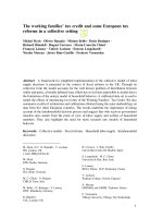
drawal rates of the other means tested benefits. Figure 1 presents the budget constraint,
which results from the interaction of the different elements of the UK tax and benefit
system for a one earner family with one child. The family receives the universal Child
Benefit, and depending on the number of hours worked, is eligible for various levels of
means tested support. The figure shows that for a large range of hours of work, the
effective marginal tax rate is close to 100% (and exceeds 100% at around 32 34 h of
work). This is a result of overlapping tax/National Insurance rates and withdrawal rates of
means tested benefits. Obviously, the more means tested benefits an individual or family is
eligible for, the more likely the problem of high marginal tax rates is going to be due to an
overlap of withdrawal rates of benefits as income rises.
Budget constraints with high marginal tax rates over a long range of hours, similar to the
one presented in Fig. 1, will be common among households with low levels of wages and
high levels of eligibility. How much means tested and in work support households can
receive is determined by three factors:
• the level of savings all means tested benefits and Family Credit are limited to

households with low levels of savings (£8000 for Income Support/JSA and Family
Credit and £16000 for Housing Benefit and Council Tax Benefit),
• whether households live in owned or rented accommodation Housing Benefit is
limited to those who pay rent,
• the number and ages of children in the household as the value of all elements of means
tested support and the Family Credit are conditional on household structure.
Therefore households with children, living in rented accommodation, and with low
level of savings are most likely to face very high marginal tax rates. Given the criterions
for eligibility to the different schemes and the make up of the UK population in 1998, a
large fraction of the labor force faces very high marginal tax rates over substantial ranges
of hours worked. In 1998/99, there were about 33 million of working age adults in
Britain. Of these, over 6 million were in receipt of some form of means tested support,
which means that they faced a marginal tax rate of at least 65%.
4
The 6 million benefit
recipients is the lower bound of the number facing weak incentives to work. On top of
the number of households who actually received support, there are those who were not
entitled because of the level of their earned income but who would receive support at
some lower level of hours worked. Taking the example of the budget constraint in Fig. 1,
at 40 h of work the level of net earned income implies that the family would not be
entitled to claim any means tested support. Yet, clearly the problem of weak work
incentives still applies.
4
In 1998, this was the lower withdrawal rate of means tested support (applied to Council Tax Benefit and
Housing Benefit). For a detailed breakdown of the number of families on means tested benefits, see for
example: Brewer, Clark, and Wakefield (2002), Department for Work and Pensions (2001).
1
5
2.3.2. Working Families’ Tax Credit
In 1998, the Labour Government announced that the Family Credit would be replaced by

the Working Families’ Tax Credit. One of the issues the reform was to address was the
problem of high marginal tax rates which resulted from the combination of income tax,
national insurance contributions and the withdrawal of Family Credit, often combined with
the withdrawal of the means tested Housing Benefit and Council Tax Benefit. The WFTC,
introduced in October 1999, builds on the Family Credit (its structure, elements and
operation are essentially the same) but it is substantially more generous.
The WFTC reform comprised increases of the applicable amount and specific credits.
5
The withdrawal taper was reduced from 70 to 55 per cent. In addition, in an attempt to
reduce the stigma associated with claiming in work support and thereby increase take up,
as well as to strengthen the link between work and the transfer, it was originally planned
that WFTC would be paid through the wage packet to the main earner rather than directly
to the main carer as in the case of FC. This part of the reform raised concern over a ‘‘purse
to wallet’’ transfer of money within couples and on its introduction couples have been left
to choose whom the WFTC is paid to.
6
Figure 2 shows the effect of WFTC (without childcare) compared with FC for a one
earner family with one child at various hours of work. Although WFTC is a much more
£0
£50
£100
£150
£200
£250
£300
0 101520253035404550
Hours worked per week
Weekly disposable income
Child Benefit Net earnings Income Support
Family Credit

Housin
g
Benefit Council Tax Benefit
5
Fig. 1 The 1998/99 fiscal system one earner couple with a child aged under 11. Notes: Gross hourly wage
of £7.00 (€10.17) the 25th percentile wage for a man in couples with children; assumed rent is £52.25
(€75.89) per week, the median rent for couples with children
5
In Table A2 in the Appendix, we present the difference in values of credits and applicable amounts
between Family Credit in April 1998 and WFTC in June 2001. Values from June 2001 include several
increases in the generosity of WFTC introduced after October 1999.
6
WFTC includes also a generous childcare credit equivalent to 70 per cent of childcare costs up to a rather
generous maximum. This is available to single parents and couples conditional on both partners working at
least 16 h a week. The maximum amount of childcare credit is 70 per cent of childcare costs up to £100 for
people with one child and up to £150 for those with two or more children. Under FC, there was an income
disregard of £60 per week on childcare expenditure. Take up of child care related financial support has been
low under both FC and WFTC and we do not include this part of the reform in our modeling. For details of
how childcare support changed between Family Credit and WFTC see for example, Myck (2000).
1
6
generous system, a lot of the difference is clawed back through reduction in Housing
Benefit and Council Tax Benefit. While WFTC increases net income at all hours of work/
earnings levels, it is interesting to note that the reform has had the highest impact (in
absolute terms) on the net incomes of those who would be just at the end of the FC taper.
Due to the WFTC’s increased generosity and reduction in the taper rate, a lot of people
who would not be eligible to claim FC because of their income level became entitled to
claim WFTC. As a consequence the government expected a near doubling of the number of
recipients of WFTC compared with FC. The reality of WFTC turned out not far off this
expectation. While in November 1998 around 800 000 families received the Family Credit,

by November 2000, i.e. a year into the WFTC reform, the number of claimants had
increased to just over 1.1 million and reached almost 1.4 million families by November
2002 (see Inland Revenue, 2002).
Since 1998/1999, apart from the WFTC, many other changes have been made to the
structure of taxes and benefits in the United Kingdom. These have been described in detail
elsewhere (for example: Adam & Kaplan, 2002; Kaplan & Leicester, 2002; Myck, 2000),
and shall not be taken into account here.
2.4. Modeling the WFTC reform
The WFTC increased the generosity of in work transfers and changed the withdrawal taper
of the transfer. Although, when eventually introduced it allowed couples to choose the
person who would receive it, the initial proposal was to pay it in all cases to the main
earner in each couple. This part of the reform would represent a significant shift of
resources from main carers (in most cases mothers) who used to receive the Family Credit
to main earners (in most cases fathers). Within the unitary framework, we would only be
able to examine the effects of increased generosity of payments, but because the collective
framework allows the analysis of the impact on choices of changes in the distribution of
resources between partners, we will also be able to consider this aspect of the reform.
£0
£50
£100
£150
£200
£250
£300
£350
01020304050
Hours worked per week
Weekly income in £
60
gross @ £7.00 Baseline - with FC

Reformed - with WFTC Difference between WFTC and FC
Fig. 2 Budget constraint for a one earner couple with child, for a gross hourly wage rate of £7.00, baseline
(April 1998) and reform systems (Working Families’ Tax Credit) Notes: See notes for Fig. 1. Net weekly
income presented for two tax and benefit systems; gross weekly income presented for reference
1
7
We will analyze two hypothetical versions of the WFTC reform:
• WFTC1: increased generosity of the payments with no change of recipient (payments
going to the main carer),
• WFTC2: increased generosity of payments with change of recipient from main carer to
main earner.
3. The data
We use individual labor force data from the UK. We calibrate a collective model of
household labor supply on couple data, in the way described by Vermeulen et al. (2006),
and predict work hours according to the model. It is this predicted hours data (our ‘‘col
lective’’ data) which we then use to simulate fiscal reforms. We first describe the UK labor
force data, then report the results of two of the steps of the estimation and calibration
exercise, namely the analysis of bargaining power inside couples and of the leisure
interaction term in couples’ preferences, as they are specific to the UK situation. We end
this section with a description of the distribution of hours worked as predicted by the
collective model.
3.1. The UK labor supply data
The data comes from the 1998/99 Family Resources Survey (FRS), which contains 22,999
households. The survey collects data on an individual basis on education, weekly hours of
work, gross weekly earnings, investment income, as well as on a range of demographic
characteristics. Other sources of income are recorded at the benefit unit (family) level.
These are mainly government transfers: Income Support, Family Credit, Housing Benefit,
sick and maternity pay, maintenance income, as well as the value of in kind benefits (e.g.
free school meals). From weekly hours of work and gross earnings we calculate gross
hourly wages. We use two sub samples of this data set:

• a sample of 1730 single individuals without children (922 men and 808 women) this
sample is used to estimate singles’ preferences,
• a sample of 4358 couples (1739 couples without children and 2619 couples with one or
two children) this sample is used for estimation of labor supply models for couples
and simulation of the WFTC reform.
The samples only include one benefit unit households and are limited to individuals
aged 25 55. We exclude any individual or couple in which either of the partners is self
employed, receives contributory Job Seekers’ Allowance (the UK unemployment benefit),
is retired or disabled, as we want to exclude households with individuals who are invol
untarily out of work. We also excluded households with disabled children, and those with
any adults in full time education and in the army. Households with more than two children,
individuals with wages above £50 (€72.62) an hour and those with missing education
information have also been excluded.
7
Table A4 in the Appendix provides summary
statistics.
7
The WFTC reform only affects households with children. Our sample therefore includes households with
children, where we limit the number of those to two, in an attempt to limit the potential effects of labor
supply constraints which are not directly related to financial gains to work.
1
8
3.2. Estimation and calibration of a collective model
To go from the data described above to the collective data used to study the impact of
fiscal reforms, we take the following steps. Firstly, we estimate parameters of prefer
ences for leisure and consumption on the sample of singles.
8
We then turn to couples,
whose preferences are assumed to be identical to those of singles, save for a term
capturing the marginal utility of the leisure of each individual’s partner. We assume

that decisions of individuals in couples are Pareto efficient. We need to estimate the
preference parameter on the leisure interaction term, together with the parameters of a
function describing the bargaining power, or which point a household chooses on the
Pareto frontier. We use both calibration and estimation to achieve this. As described
in Vermeulen et al. (2006) in the first stage of calibration we obtain values of the
man’s welfare weight (l
m
) and the parameter on the interaction of leisures in the
individual utility functions of partners (d). l
m
is defined as in Eq. (8) of Vermeulen
et al. (2006):
l
m
k
Ã
d
Ã
ðÞ=K; ð1Þ
where K is the number of discretized points between the man’s maximum and minimum
utility levels for an optimal d=d
*
, and k
*
is the optimal point between the two extremes.
9
In the second stage we estimate a linear equation on the calibrated man’s welfare weight
and using predictions from this equation
^
l

0
m
ÀÁ
recalibrate the d.
10
For each household, we
then predict the optimal consumption leisure choice, given the values of all parameters of
the system. This data set of predicted optimal choices is the collective data set which we
use to perform the fiscal reform simulations.
Before turning to the simulation of the reform we present the analysis of bargaining
power and leisure interaction terms for the UK.
3.2.1. Bargaining power
We allow for bargaining power within households, as captured by the man’s welfare
weight l
m
, to depend on relative wages (difference in gross wages between the man and the
woman), relative investment income (difference in gross investment/savings income be
tween the man and the woman), relative unearned income and on the earning potential
implied by the tax and benefit system. From the point of view of the collective framework
these variables (distribution factors) are crucial determinants of the distribution process.
Bargaining power in our model also depends on the difference in age and education, and
the number and ages of children (see, for example, Bourguignon, Browning, Chiappori, &
Lechene, 1993).
The relative earning potential implied by the tax and benefit system is defined as:
8
For results of the estimation of the parameters of single individuals’ utility functions see the Appendix
(Table A3).
9
We shall use interchangeably the terms ‘‘bargaining power’’ and ‘‘welfare weight’’, in order simply to
avoid tedious repetitions. But note that due to the nonconvexity of budget sets the welfare weight does not

correspond to a linear combination of spouses’ utilities.
10
In this application of the Vermeulen et al. (2006) methodology we do not allow d to be different for men
and women, and we use calibrated rather than predicted values of d.
1
9
P
X
K
k 1
ðR
f 40
mk
R
f 0
mk
Þ
X
L
l 1
ðR
fl
m40
R
fl
m0
Þ
"#
=100; ð2Þ
where R

fl
mk
is the total household income where the partners’ labor supplies correspond to
the lth and kth discretized hours bracket (respectively of the woman and the man). The
hours distribution is discretized into K and L hour brackets.
11
Earning potential is thus the
difference between the man’s and woman’s contribution to the (net) household income,
where the contribution is calculated as the sum of differences between incomes at 40 and
0 h of work of the partner over a number of hours brackets K or L. If the tax and benefit
system changes in such a way that it increases the man’s contribution relative to the
woman’s, the value of the variable will increase. Such definition of the relative earning
potential is a slightly simpler specification of the one suggested in Eq. (12) of Vermeulen
et al. (2006), but its interpretation is essentially the same. The variable measures how much
net income the female in the couple contributes to the household budget relative to the
man’s contribution, once we take account of the tax and benefit system and of the hours’
options the partners can choose from.
From the formulation of the earnings potential variable presented above it should be
obvious that it does not account for different forms of administration and payment of taxes
and benefits. Yet precisely this aspect is central to analyzing the effects of the WFTC
reform. Here we therefore include an additional variable which accounts for the distri
bution of unearned income. The variable, which is an additional distribution factor, is
defined as the relative woman’s unearned income at 40/0 h worked, and takes the
following form:
Y
UN
f
F
f 0
m40

=R
f 0
m40

à 100; ð3Þ
Y
UN
f
is the ratio of woman’s unearned income, F
f 0
m40
, to total couple’s income, R
f 0
m40
;
when the man is working 40 h and the woman is working 0 h.
12
This specific hours
combination has been chosen given the rules determining in work support. At this com
bination of hours most low income couples with children will still be eligible for FC and/or
WFTC and the value of the variable should therefore change with changes in their gen
erosity and administration. The variable, among other things, will allow us to capture the
difference between the two versions of the WFTC.
Table 1 presents results of a simple (linear) regression of the male welfare weight, w
m
,
on the four distribution factors: P, Y
UN
f
; the difference between his and her gross wage,

and the difference between his and her investment/savings income, and on a vector of other
characteristics.
Living in London and having a child aged 0 4 negatively influences the male bar
gaining position. Men who are better educated than their partners have less bargaining
power than men who have either the same educational level or less, and the larger the
difference in ages between the man and the woman, the lower the man’s bargaining power.
These last results go in the opposite direction of what has been found in most studies for
other countries in this project. One of the possible explanations for these findings is the fact
11
We split both the male and the female hours distributions into 7 h brackets: 0 5, 6 15, , 45 55, 56+, and
calculate net incomes for these brackets respectively at: 0, 10, , 50 h and 60 h of work. The value is
divided by 100 for numerical and presentational reasons.
12
The scaling is again guided by the reasons given in Footnote 11.
1
10
that, as mentioned by Vermeulen et al. (2006, Sections 3.1 and 3.2), our model ignores
household production, and considers all nonlabor time as pure leisure.
13
This implies that a
situation in which the woman is not employed but the man is, or in which the woman
works less than the man, is interpreted as a reflection of higher bargaining power of the
woman (since she is treated as having more leisure). In many such situations women may
in fact spend considerable amount of their nonlabor time on household work and childcare,
and this would presumably be more likely in couples where the man is better educated and
older (and thus relatively more ‘productive’ on the labor market). It is therefore possible
these counterintuitive effects could disappear if we treated household production explicitly
in the model. Our finding thus stresses the importance of extending the model to include
household production. On top of this one could also argue that because the socio
demographic characteristics determine both the bargaining power and either preferences or

the budget constraint (or both) there is no obvious a priori expectation concerning the
direction in which they would affect the bargaining position in the household.
14
The coefficients on the distribution factors, except for the coefficient on the difference
between his and her investment income, have the expected signs. Higher gross wage of the
man relative to the gross wage of his partner, higher earning potential (P) and lower values
of female unearned income Y
UN
f

all imply a higher bargaining power of the man. In
Table 2 we present summary statistics for the calibrated and estimated values of the
parameters of the collective model: men’s welfare weight, l
m
, and the coefficient on the
Table 1 Determinants of men’s welfare weight a linear regression
Dependent variable: Men’s bargaining power: l
m
Coefficient SE
Constant 0.582** (0.005)
Difference in age 0.002** (0.001)
Dummy variables for difference in education
Man’s education 1 levels higher 0.007 (0.008)
Man’s education 2 levels higher 0.039** (0.015)
Man’s education 1 level lower 0.024** (0.007)
Man’s education 2 levels lower 0.032** (0.014)
Youngest child aged 0 4 0.024** (0.006)
Youngest child aged 5 10 0.020** (0.007)
P 0.014** (0.002)
Y

UN
f
0.007** (0.000)
Difference in gross wage 0.034** (0.004)
Difference in investment/savings income/100 0.027** (0.009)
Living in London 0.043** (0.008)
Number of observations 4358
Adjusted R
2
0.1915
Notes: Difference in age: his age minus her age. Dummy variables for education: level of education
determined by the age when left full time education. Individuals are divided into three education groups: left
school aged 16 or less, left school aged 17 or 18, and left school aged 19 or more. Dummy for ‘Man’s
education 2 levels higher’ takes value 1 if man left education aged 19+ and woman left education aged 16 or
less. On the other hand, ‘Man’s education 1 level lower’ take value one if either: woman left education aged
17 or 18 and man aged 16 or less, or if woman left education aged 19+ and man aged 17 18. The omitted
education category is couples where both partners have the same level of education. The omitted youngest
child category is youngest child aged 11 18. Difference in gross wage: his gross wage minus her gross
wage. Difference in investment/savings income: his investment/savings income minus hers. (**) implies
significance at 5%
13
See Vermeulen et al. (2006) for some qualification of this statement.
14
See Section 6 for results obtained for other countries.
1
11
interaction of leisure terms in the utility function, d. Relative to the calibrated value of l
m
there is much less variation in the estimated parameter.
3.3. The collective data set

Each observation in the collective data set corresponds to a household for which the hours
of work of the two adult members have been predicted using the collective model (with
estimated bargaining power and leisure interaction terms). Household income is also
predicted given wages, unearned income and predicted hours of work. To assess the quality
of our prediction, we compare the distributions of hours in the data and as predicted by the
model.
We find that predicted hours and actual hours coincide for 51.0% of men and 56.1% of
women, and that for a further 41.4% of men and 36.4% of women, the prediction is within
1 h bracket of the actual number of hours worked. Table 3 shows the percentage of
observations in each of 7 h brackets, for numbers of hours worked, both actual and as
predicted by the collective model. Overall, the model’s predictions are not far off from the
actual distribution of hours worked. For both men and women the model underpredicts the
proportion working between 36 and 45 h per week, which is the most common observed
combination of hours worked.
4. Theoretical effects of a reform of the tax and benefit system
We discuss the theoretical effect of a reform such as that of in work transfers implemented
in the UK in 1999, both in the unitary and the collective frameworks.
Table 2 Summary statistics for calibrated and estimated parameters of the collective model
Mean Standard deviation Min. value Max. value
Calibrated l
m
0.565 0.181 0 1
Estimated l
m
0.565 0.080 0.094 0.973
Calibrated d 0.066 0.361 0.9 4.0
Table 3 Hours distributions: actual and collective predictions
Men Women
Actual (%) Predicted (%) Actual (%) Predicted (%)
Hours bracket

From 0 to 5 3.1 1.9 16.4 14.4
From 6 to 15 0.2 0.3 7.1 12.8
From 16 to 25 0.7 1.4 17.9 19.7
From 26 to 35 1.4 2.6 13.9 19.5
From 36 to 45 44.3 27.6 33.0 23.2
From 46 to 55 32.2 53.2 8.9 8.4
Above 56 18.3 13.2 2.7 2.3
1
12
As we mentioned above, the 1999 WFTC reform has two important aspects. Firstly, it
represents an increase in generosity of in work support for families with children, and
secondly it introduces an option of payments via the pay packet.
15
The first element of the reform increase in the value of in work benefit expands the
opportunity set for those couples with children who at some combination of hours worked
would potentially be eligible to claim WFTC. Because of conditions restricting eligibility
for in work support, some couples with children will not see a change in their budget
constraint. Increased generosity of the payments will not affect:
16
• households with levels of savings which make them ineligible to claim WFTC,
17
• households where wages of both partners are so high that even at the minimum required
level of hours the couple is not eligible to claim any WFTC.
The second element of the reform, the option of payment via the pay packet, is not
innocuous. Indeed, to the change in payment mode can be associated a change in identity
of recipient within the household, and this in turn may lead to behavioral changes for a
given level of the transfer.
4.1. Effect of the WFTC reform in the unitary framework
Since the unitary model implies that household resources are pooled, in such a framework
the amount of a transfer but not the identity of the transfer recipient influences household

choices. Therefore, in a unitary framework, whether the WFTC is paid to the mother or to
the main earner will have no effect on behavior, and thus households will respond in the
same way to both variants of the reform we consider, which both amount to an increase of
non labor income. If leisure of both household members is normal, labor supply should
decrease, and the extent of the decrease will depend on the relative marginal utility of
leisure and of other goods in the household preferences. We can expect larger effects if
individual wages are very different, with the low wage partner more likely to leave work.
Finally, because receipt of the WFTC is conditional on at least one person working 16 h,
we should not see any couple with at least one person in work prior to the reform become a
‘workless’ family.
An important feature of the unitary model is the fact that potentially higher incomes in
‘sub optimal’ scenarios have no effect on the final decision. This means that any change in
labor supply will take place only among those who following the reform actually end up
claiming the WFTC. In other words, if in the baseline and reform systems the highest level
of utility is achieved at a point where the household is not eligible to claim any FC/WFTC,
then the fact that they could claim it at some different level of hours worked will not affect
their behavior. In the unitary framework, if couples change their behavior following the
reform, the new optimum has to be at a point where they receive some WFTC. As we shall
see below, this is not necessarily the case in the collective model.
15
Note that the WFTC retains the conditionality of the transfer on a minimum number of hours worked
(16 h per week worked by either member) as in its predecessor, the Family Credit.
16
Out of 2619 couples with children in our sample, the budget constraint is unchanged by the WFTC for 676
couples.
17
WFTC is restricted to those with savings less than £8000. Eligibility is reduced (by £1 for every £250 of
savings) for those with savings above £3000.
1
13

4.2. Effect of the WFTC reform in the collective framework
Households behaving collectively will be affected by a broader set of reforms than unitary
households. Indeed, collective households will not only react to reforms which change total
income, but also, potentially at least, to reforms which modify any of the arguments of the
intra household bargaining power. Typically, bargaining power depends on relative wages
or relative earning potential. For the UK, recall that we found bargaining power to depend
significantly on differences in gross hourly wages and investment income, unearned in
come of the woman relative to overall income at the 40 0 (his her) combination of hours
worked, and on the earning potential implied by the tax and benefit system.
From the perspective of mechanisms through which relative earning potential and
distribution of resources influence behavior in couples in the collective model we can
distinguish three types of tax and benefit reforms:
1) Reforms which only affect the distribution of resources but not their overall level: an
example of this is a hypothetical reform of the Child Benefit, with change in the
identity of the recipient and constant amount of benefit. Such a reform affects neither
the Pareto frontier nor the contributions to the household’s income (captured in our
setting by the P variable). In our model, the only way such a reform affects the
distribution of resources within the family is via the ratio of unearned income of the
woman to the total household income (i.e. Y
UN
f
variable).
2) Reforms which affect both the Pareto frontier and the distribution of resources within
households. In the light of our model, we can distinguish two types of such reforms:
a. reforms which do not affect the distribution of unearned income (as summarized
in the Y
UN
f
variable),
18

b. reforms which change both the relative contributions to the household’s income
(P) and have an effect on the distribution of unearned income Y
UN
f

.
Most fiscal reforms, including the WFTC reform, fall into the last category. For
households who would be potentially eligible for the WFTC, the reform changes the shape
of the Pareto frontier, as well as the relative contribution to the household budget P, and
for many couples with children, it affects the level of the female unearned income to total
household income. Because of the last effect we expect to see a difference in the response
to the reform depending whether in work support is paid to the main carer or the main
earner.
Unlike in the unitary framework, where the reform affects household behavior only
through changes in the family budget constraint, response to the WFTC in the collective
framework will be a combination of two effects: responses to changes in the Pareto frontier
and to changes in the relative bargaining power resulting from different values of P and
Y
UN
f
: The implication of the change in the bargaining power is that in the collective
framework, we might observe changes in behavior of couples who neither before nor after
the reform claim any in work support. We analyze below what the likely effects of the
reform are in terms of labor supply decisions and how the reform will influence the relative
bargaining power of the partners.
18
It is difficult to think of an example of such a reform in the case where we define the distribution of
unearned income relative to overall net family income. Any reform affecting net incomes would change the
value of the variable summarizing this distribution even if absolute values of unearned incomes remained
unaffected.

1
14
4.2.1. Changes in bargaining power
Two of the distribution factors we consider which could be affected by the WFTC reform
are the earning potential variable, P, and the ratio of unearned income of the woman to
total household income at the 40 0 h combination, Y
UN
f
.
4.2.1.1. WFTC and the earning potential variable. Because the P variable measures the
contributions to the overall household income and disregards the way income is distributed
between partners, its value will be the same regardless of who receives the WFTC. The
WFTC reform will affect the value of P, since the reform changes the household budget
constraint, but the value after the reform will be the same for WFTC1 and WFTC2. Since
the reform potentially increases the contribution of each partner to the household income,
the earning potential variable can either increase or decrease, depending on which
contribution increases most. It is therefore ambiguous how the bargaining power of the
partners will change as a result of increasing the generosity of in work support.
Consider the effect of the WFTC reform on the earning potential variable P. The reform
increases the amount of in work support which the couple receives at combinations of
hours worked at which their level of income makes them eligible for it. For the moment, it
is not relevant who receives the payments, since we are concerned with contributions of
each of the partners to the overall household income.
The increased generosity of payments will affect the difference in the household income
between working and not working given the labor supply of the partner, i.e. for the man the
value of: R
fl
m40
R
fl

m0
and the woman the value of: R
f 40
mk
R
f 0
mk
(see above). Focusing on
R
fl
m40
R
fl
m0
it is unclear whether this difference will be positive or negative. Because
WFTC is means tested, we would expect the reform to increase R
fl
m0
(if fl>16 to make the
family eligible for the WFTC) by more than it increases R
fl
m40
. However, Fig. 2 shows that
this does not have to be the case: the highest increase in household income occurs at a
relatively high level of hours worked. This will be the case especially if the man’s wages
are low enough to make the couple eligible for WFTC in the scenario when he works 40 h.
The difference: R
fl
m40
R

fl
m0
will therefore be likely to increase (thus reducing the value of
the P variable) for couples where the man’s wage is low. Similarly R
fl
m40
R
fl
m0
will be
likely to increase for couples where the woman’s wage is low.
Given the complex nature of the in work support system and the complexity of the P
variable itself, it is difficult to give more satisfactory intuition as to how the earning
potential variable should change with the introduction of the reform. It is important to
remember, though, that increased generosity of in work support does not have to imply
higher bargaining power of either the man or the woman.
4.2.1.2. WFTC and the expected ratio of unearned income of the woman to total household
income. The value of the Y
UN
f
variable will change as a result of the increased gen
erosity of in work support and it will differ depending on the recipient of WFTC payments.
It will be lower when the transfer is paid to the father rather than to the mother. Since the
WFTC2 reform gives the payment to the main earner (and in the 40 0 combination of
hours it will be the father), and WFTC1 always gives it to the mother, the value of Y
UN
f
will be lower with WFTC2 than with WFTC1 for all couples eligible for in work support at
the 40 0 combination of hours. This intuitive result is corroborated by the negative sign of
the coefficient on the Y

UN
f
variable in the estimation of the bargaining power equation
1
15
(Table 1). The comparison between men’s bargaining power under WFTC1 and WFTC2 is
unambiguous: men’s bargaining power is greater under the option where they receive a
higher level of transfer (WFTC2) than under the option where they do not (WFTC1).
This does not mean however that following the WFTC2 the bargaining power of the
man will be higher than under the base tax and benefit system with Family Credit. The
positive effect on the man’s bargaining power of changing the recipient of in work support
can still be outweighed by a possible negative effect of the reform on the earning potential
variable P . It is therefore difficult to give a clear cut prediction of the effect of the
introduction of the WFTC (in either of its variants) on the bargaining position of house
holds.
4.2.2. Changes in households’ labor supply
The outcome of the reform in terms of labor supply decisions of individuals in couples is
less obvious in the collective framework than it is in the unitary model. Let us consider the
potential effect of an increase in the bargaining power of the man as a result of changing
the distribution of resources between partners, for a given level of transfer. In the
framework of our model, this would have a straightforward positive effect on the bar
gaining power of the man in all couples with children, without changing the highest
U
m
max
ÀÁ
and lowest U
m
min
ÀÁ

levels of utility he can achieve. Our model then allows the
woman in each couple to find the highest level of her utility conditional on the utility of her
partner satisfying the condition:
U
m
ðc
m
; l
m
; l
f
Þ!U
m
min
þ
^
l
R
m
ðU
m
max
U
m
min
Þ; ð4Þ
where
^
l
R

m
is the predicted value of the man’s welfare weight in the reformed system. To
find the optimal solution, we do a double grid search on both hours and share of con
sumption of the woman. At each of the 49 possible hours choices, and for each value of the
share of consumption between 0.1 and 0.9, we calculate the woman’s utility.
Therefore, depending on preferences concerning the leisure consumption trade off, an
increase in bargaining power of the man might imply a reduction in male labor supply, an
increase in the share of consumption of the man, or both. This could be (but does not have
to be) accompanied by an increase of female labor supply, a reduction in female share of
consumption, or both. Women with higher preference for leisure would be more likely to
respond by reducing their share of consumption, while those with higher preference for
consumption would be more likely to increase their labor supply.
The issue is complicated further by the fact that each individual’s utility is directly
affected by the level of his or her partner’s leisure. This implies that for example, if the
coefficient on interaction of leisure terms in the partners’ utility functions d is positive,
then an increase in his level of utility (to reflect his higher bargaining power) might be
achieved even in a situation when his leisure and consumption fall, provided her leisure
increases to compensate. On the other hand, if d is negative then higher utility of the man
can be achieved even in a situation when his consumption falls and his leisure remains
unchanged, provided that her leisure falls enough.
The above example shows that even in the case of a simple reform where we only
transfer resources between partners, it is unclear how we would expect couples to respond
in terms of changes in individual labor supply and consumption. Matters get even more
complicated once, apart from the change in bargaining power, a reform leads to a shift in
the Pareto frontier, as is the case with the increased generosity of payment in the WFTC
1
16
reform. Predicting how couples would respond to the introduction of WFTC is in our
framework extremely difficult and it seems that the framework allows the reform to lead to
outcomes which may seem rather unintuitive.

5. Effect of the WFTC reform in the collective model
We simulate the WFTC reform under the assumption that households behave as described
by the collective model which has been used to generate the data.
Below we report the results of simulations of the WFTC reform in its two forms:
WFTC1 reform where the more generous benefits are paid to the main carer, and
WFTC2 where the more generous benefits are paid to the main earner. We discuss
changes in the man’s predicted bargaining power and changes in hours choices after the
reform. We also present a brief welfare analysis.
5.1. Effect of the reforms on the man’s bargaining power
As discussed in Section 4.2, the theoretical effect of the reforms on men’s bargaining
power is ambiguous. We expect the man’s bargaining power to be greater in WFTC2 than
in WFTC1, but recall that for some households it could decrease with both reforms.
Figures 3 and 4 show that the two versions of the reform have very different effects on
the bargaining power of men, as is expected, given that men’s resources are different in
both variants. In both figures, we represent the man’s welfare weight after the reform
^
l
R1
m
À
and
^
l
R2
m
Á
as a function of the welfare weight before the reform
^
l
0

m
ÀÁ
. The line across each
figure is the 45° line. The difference between these two figures is a sole result of the effect
of the redistribution of resources from the woman to the man, which is captured by the
change in the Y
UN
f
variable. Indeed, as discussed above, changes in the earning potential
variable P (and its effect on bargaining power) are the same regardless of who receives the
payments.
Among the 2619 couples with children, relative to the pre reform level, bargaining
power changes in 1946 cases, and out of those, in 1163 couples, men’s bargaining power
under WFTC1 is lower than men’s bargaining power under WFTC2. Bargaining power
does not change as a result of the reform only for 673 couples with children. In all these
cases this is because the variables which summarize the effect of the tax and benefit system
on bargaining power are unaffected by the reform. For a large majority of these couples,
the reason is that WFTC is restricted because of high level of savings (over £8,000
(€11,620)), which makes them ineligible to claim in work support.
The first version of the reform, in which the amount of the transfer is increased with no
change in the identity of the recipient (the main carer, i.e. by default the woman), increases
the bargaining power of the woman in 1174 couples and lowers it in 772 couples. It is
interesting to note a clear pattern which emerges from Fig. 3. In couples where the bar
gaining power of the man is highest before the reform, the WFTC reform has very little
effect. Bargaining power changes most for couples with the men’s original welfare weight
at about 0.5 and below this level.
Giving the WFTC to the main earner (in our simulation always the father) results in an
increase of the bargaining power of men in 1741 couples. In 205 cases the man’s bar
gaining power is lower as a result of the reform. This happens because the earning potential
variable P changes in favor of women, which in some cases is enough to outweigh the

1
17
Man's welfare wei
g
ht: base
Man's welfare weight: base Man's welfare weight: WFTC1
0
5 1
0
.5
1
Fig. 3 The man’s welfare weight before and after the WFTC1 reform in couples with children
Notes: Man’s post reform welfare weight
^
l
R1
m
ÀÁ
on the vertical axis
Man's welfare wei
g
ht: base
Man's welfare weight: base Man's welfare weight: WFTC2
0
.5 1
0
.5
1
Fig. 4 The man’s welfare weight before and after the WFTC2 reform in couples with children
Notes: Man’s post reform welfare weight ^l

R2
m
ÀÁ
on the vertical axis
1
18
effect of redistribution of payments from ‘‘purse to wallet’’. As we can see from Fig. 4 the
loss of bargaining power by men in these situations is minimal.
5.2. WFTC1 and WFTC2: changes in participation and hours
We present the results we obtain in terms of hours and participation with both reforms, and
compare the effects of WFTC1 and WFTC2. Tables 4 and 5 present changes in hours
worked for men and women in couples with children as a result of, respectively, WFTC1
and WFTC2. In about 50% of couples, at least one household member changes his/her
labor supply following the introduction of either of the WFTC reforms. Given the fact that
we model the reform in a world with discretized and not continuous hours choices this is a
surprisingly high proportion.
19
We must remember, though, that unlike in the unitary
model, the collective framework can lead to a behavioral change even though the couple
receives no in work support before or after the reform. In fact, out of 1342 couples in
which labor supply of either or both partners changes following WFTC1 reform, only
34.5% are eligible to claim in work support given their post reform labor supplies (the
respective numbers for WFTC2 are 1253 and 40.5%). The reason for this is the effect of
the reform on the earning potential variable and the distribution of unearned income. These
changes result in different relative bargaining power irrespective of whether the couple in
the end receives the WFTC or not. Such an effect is unique to the collective model, and
cannot be captured by simulations of the reforms using the unitary specification.
Table 4 WFTC1, changes in male and female hours couples with children
Change in male hours Change in female hours
£ 20 10 0 10 ‡20 Total

£ 20 2.3% 1.9% 1.2% 0.0% 0.0% 5.4%
10 2.9% 4.7% 4.2% 1.2% 0.0% 12.9%
0 1.3% 6.5% 48.8% 7.0% 0.4% 63.9%
10 0.4% 3.9% 9.3% 1.4% 0.2% 15.1%
‡20 0.1% 0.4% 2.1% 0.1% 0.0% 2.7%
Total 7.0% 17.3% 65.4% 9.6% 0.6% 2619 couples
Table 5 WFTC2, changes in male and female hours couples with children
Change in male hours Change in female hours
£ 20 10 0 10 ‡20 Total
£ 20 2.3% 4.4% 3.1% 0.3% 0.1% 10.1%
10 1.1% 5.7% 4.9% 2.1% 0.1% 14.0%
0 0.6% 3.4% 52.2% 8.5% 0.4% 65.0%
10 0.2% 0.7% 7.1% 1.0% 0.4% 9.2%
‡20 0.0% 0.0% 1.6% 0.0% 0.0% 1.7%
Total 4.0% 14.2% 68.9% 11.8% 1.0% 2619 couples
19
If we simulated the reform in a framework which would allow modeling the choice of labor supply with a
continuous hours distribution we would expect a change in the labor supply of all couples who would see
their Pareto frontier and/or bargaining power change as a result of the WFTC.
1
19
The proportion of men in couples with children who do not change their labor supply
following the reform is slightly lower than the proportion of women who do not change
their labor supply, both under WFTC1 and WFTC2. As we expected, relative to the
response to WFTC1, under WFTC2 fewer women reduce their labor supply and more
women respond by increasing their hours of work. This comes from the fact that both
income and bargaining power of the woman are lower under WFTC2 than under WFTC1.
The converse is true for men. The proportion of men reducing their hours following
WFTC1 is almost 6 percentage points lower than following WFTC2.
Tables 6 and 7 give a summary of differences in labor supply between the two versions

of WFTC for men and for women, respectively. Although, Tables 4 and 5 suggest a
relatively high degree of similarity in the reaction to the two versions of the WFTC,
looking at how men and women respond shows a striking disparity between the results. For
24% of men and 19% of women in couples with children the reforms have a different effect
on behavior on the labor market. Given that 56% of men and 60% of women with children
do not respond to either of the reforms, this means that around a half of those who do
respond reacts differently depending on whether the WFTC is paid to the main carer or the
main earner.
5.3. Participation, consumption and welfare
In Table 8, we present an aggregate summary of the results in terms of participation,
consumption and welfare. The second column shows information for the collective data,
while the third and fourth shows aggregate values for the two WFTC simulations in the
collective world. We can see that both versions of the reform have a positive effect on male
participation. When male bargaining power increases as a result of giving the WFTC to the
Table 6 WFTC1 vs. WFTC2, changes in male hours
Change in male hours WFTC1 Change in male hours WFTC2
£ 20 10 0 10 ‡ 20 Total
£ 20 3.8% 1.3% 0.3% 0.0% 0.0% 5.6%
10 3.7% 7.0% 2.1% 0.1% 0.0% 12.9%
0 2.1% 4.7% 56.1% 1.1% 0.0% 63.9%
10 0.5% 1.0% 6.0% 7.5% 0.2% 15.1%
‡ 20 0.0% 0.1% 0.6% 0.5% 1.5% 2.7%
Total 10.1% 14.0% 65.0% 9.2% 1.7% 2619 couples
Table 7 WFTC1 vs. WFTC2, changes in female hours
Change in female
hours WFTC1
Change in female hours WFTC2
£ 20 10 0 10 ‡20 Total
£ 20 3.0% 2.4% 1.5% 0.1% 0.0% 7.0%
10 0.8% 9.7% 6.2% 0.5% 0.0% 17.3%

0 0.2% 1.8% 59.6% 3.5% 0.3% 65.4%
10 0.0% 0.2% 1.6% 7.6% 0.2% 9.6%
‡ 20 0.0% 0.0% 0.0% 0.1% 0.5% 0.6%
Total 4.1% 14.2% 68.9% 11.8% 1.0% 2619 couples
1
20
main earner, the effect on male participation is lower than when WFTC is paid to the main
carer (men have more bargaining power, hence increase participation less). The reverse is
true for women. The changes in participation following the reforms imply that under
WFTC2 there is a higher number of workless couples. On average male consumption falls
under WFTC1 and female consumption falls under WFTC2.
An important advantage of the collective model is the possibility to analyze changes in
the individual levels of utility. As Table 8 shows on average utility of women increases
under WFTC1 and falls under WFTC2 and the reverse is true for average utility level of
men.
20
However, neither of the versions of the reform unambiguously increases the utility
of all men or all women. Because of the effect of increased generosity of payments
between Family Credit and WFTC, and the resulting changes in bargaining power, both
variants of the reform have positive and negative effect on utility of men and women.
In Table 9, we present a summary of changes in utility levels. About 42.5% of couples
with children are not affected by the WFTC1 reform and at all. This proportion is higher (at
49.7%) in the case of WFTC2. This may be because the couples are not eligible to claim
Table 8 WFTC reforms couples with children
Collective data WFTC1 WFTC2
Participation
Men 97.8% 99.1% 98.7%
Women 81.1% 73.7% 75.5%
Hours of work
Men 47.5 46.6 44.6

Women 26.9 26.7 27.8
Proportion of families
No one in work 2.2% 0.9% 1.2%
Only woman in work 0.1% 0.0% 0.1%
Only man in work 16.7% 25.4% 23.4%
Both in work 81.1% 73.7% 75.4%
Consumption
Men 239.0 233.9 242.9
Women 299.9 303.1 292.1
Utility
Men 37.8 37.5 38.0
Women 48.0 48.3 47.8
Table 9 Individual level welfare analysis of the WFTC reform
WFTC1 WFTC2
Change in Um Change in Uw Change in Um Change in Uw
0+ 0+
0.0 0.0 37.3 0.0 0.0 2.8
0 0.0 42.5 0.0 0 0.0 49.7 0.0
+ 16.8 0.0 3.3 + 37.4 0.0 10.1
Notes: Figures in percentages of couples with children. Um man’s utility, Uw woman’s utility
20
Note that the interpretation of aggregate changes in utility requires some caution as averaging across
individuals and households implies cardinalization of utility. However, we use these average figures only to
reflect differences between the three systems and we think that these reflect the implications of the two
versions of WFTC.
1
21
any WFTC or because changes in the budget constraint and/or bargaining power are so
small that the individual levels of leisure and consumption are unaffected in our discretized
approach. WFTC1 positively affects utility of both men and women in only 3.3% of

couples with children, WFTC2 in 10.1%. Differences between the two variants of the
reform come out especially when we look at the proportions of couples where one partner
gains and the other looses. Following WFCT2 the proportion of couples where the man
gains and the woman loses is 37.4% which is almost double the figure under WFTC1. On
the other hand, if the more generous payments are given to the mother, in 37.3% of couples
with children the woman’s utility level increases and the utility of her partner falls.
21
6. Summary of comparable results for five other European countries
Similar analysis was conducted for reforms of the tax and benefit systems in Belgium,
France, Germany, Italy, and Spain.
22
The papers use the same or very similar methodology
(described in Vermeulen et al., 2006), but are applied to different reforms and based on
country specific data. Below we present a summary of results from these studies. In the
description of these results we focus on the determinants of the relative bargaining power,
the nature of modeled reforms and on some key effects they bring about. As far as
determinants of bargaining power are concerned, the signs of the estimated coefficients are
given in parentheses.
6.1. Belgium
The distribution of the woman’s estimated power index has a mean of .62, but is very
asymmetric, as it is approximately unimodal with mode near .94. Significant determinants
are her expected marginal contribution to household disposable income when switching
from 0 to 40 h worked per week (+), his corresponding expected increment when switching
from 30 to 40 h ()), her minus his unearned income (+), total household unearned income
(+), living in Brussels ()), higher education indicators (both his and her )) and white collar
indicators (his +, her )). Note that the variables with a direct ‘‘collective’’ interpretation
have the expected sign.
The reform currently implemented (henceforth ‘‘Belgian reform’’) consists of four main
measures: (i) introduction of a repayable tax credit for low earnings; (ii) changes in tax
brackets and lowering of the two highest marginal tax rates from 55% and 52.5% to 50%;

(iii) equalization of tax exemption of married and single individuals; (iv) extension of
marital quotient to couples with a cohabiting contract. A linear taxation system is also
modeled, with a negative income tax component. The slope is set to 50%, and for the
intercept, the value is set so as to obtain revenue neutrality as far as taxes and social
security contributions are concerned. This leads to a yearly minimum guaranteed income
of 2,900 euro per person.
21
As mentioned in Footnote 6 the WFTC reform included a more generous treatment of childcare expenses
for working families. This part of the reform in not modeled here. Initially take up of the childcare tax credit
was very low, so excluding it from our analysis should not distort the results too strongly. However, with the
signs of increases in the take up of childcare related credits it seems that any future analysis of the effect of
tax credits on labor supply should account for childcare expenses and the related subsidies.
22
For references see Vermeulen et al. (2006).
1
22
The Belgian reform improves the bargaining position of a majority of women. Col
lective labor supply reactions to the reform are moderate, with more than 90% of indi
viduals retaining their baseline situation, both for men and women. When there is
movement it is on average a slight decrease in labor supply. The linear taxation has an
adverse effect on the bargaining position of most women, especially at lower levels. Here
again, labor supply reactions are moderate when predicted with the collective model. Most
changes concern people leaving the labor force as a consequence of the introduction of a
relatively high minimum guaranteed income. According to the collective model, the reform
is a Pareto improvement for about 30% of the households, disadvantages both spouses for
some 20%, and has conflicting impacts for 46%. The reform increases overall inequality,
leaving the concentration ratio almost unchanged.
6.2. France
Although, the French study concentrates on the man’s negotiated utility rather than on the
power index used in other studies (see Vermeulen et al., 2006, Section 3.3.1), it also reports

the latter, and we focus on it here for ease of comparison. The calibrated power index for the
man has a bimodal distribution, with modes at .35 and .84, and it ranges over the whole [0,1]
interval. Variables with a significant impact in the prediction of the man’s negotiated utility
are the minimum utility level (corresponding to a dictatorial position for the wife) and
interactions of the difference between maximum and minimum utility levels and the man’s
expected relative earning power (+), the age difference (his minus her: +), the difference in
education level (his minus her: )), the overall number of dependent children (+), the number
of older dependent children (aged 12 15: )), and the difference between unemployment rates
relevant to each individual, depending on sex and education level (his minus her: )). Note that
with a coefficient of 1 for minimum utility, this specification coincides exactly with a linear
regression of the male’s power index on the list of variables interacted with the utility range.
Since the estimated coefficient is very close to 1, comparability with the results from other
studies is directly warranted. The baseline situation retained corresponds to calibrated values,
but with retention of residuals from the estimation of the man’s negotiated utility level, in
order to trace changes to that magnitude as a consequence of the reform.
The specific reform studied for France consists in a tax credit for low wage earners, and
its objectives are to provide incentives to work, and to subsidize low earnings. It is thus
similar to the WFTC reform discussed above for the UK. Due to the importance of the
inactivity trap, only 22% of the couples in the sample have a convex utility set.
Although, the Pareto frontier shifts towards the North East for about half of the
households (efficiency effect) the final effect on the man’s negotiated utility is negative on
average: this is caused by a decrease in the expected relative earning capacity of half of the
husbands (it increases for only 25%).
The effects of the reform on labor supplies, as predicted by the collective model, are
rather small, with only 5% of wives and 1% of husbands altering their labor supply. Note
that about 10% of these are not recipients of the tax credit after the reform: this type of
reaction is purely ‘‘collective’’, and is ruled out by the unitary setting.
6.3. Germany
Only 42% of the couples turn out to have a convex utility set. The calibrated male power
index has a mean of 0.45, and its significant determinants, in separate regressions for East

1
23
and West Germany, are the woman’s relative earning power at 40 h of work (), with a
larger absolute value in the West), and the age difference (her minus his: +, only in the
West). The predicted male power index has a fairly stable mean of .45 in all situations, and
its range is also stable, from about .27 to .53.
Three reforms are considered:
i) The ongoing tax reform (henceforth ‘‘German tax reform’’) mainly concerns the tax
rates applied: in this respect it is more generous than the baseline 1998 tax system, with
the basic rate reduced to 15%, from 7500 euro on, and the top rate to 42%, from 5000
euro on. But the modeling here exaggerates the generosity of the reform by ignoring
the suppression of various tax exemptions, for lack of the underlying information.
Child benefits and allowances are increased.
ii) A move from joint to individual taxation is modeled on the basis of the 1998 tax
schedule and existing benefits, with tax liabilities scaled down by the factor 0.95 in
order to obtain overall tax neutrality, i.e. keeping fixed the net revenues of the state
from the complete tax benefit system.
iii) A move to linear taxation, keeping joint taxation of couples. This is defined with a
negative income tax of about 6,000 euro for singles and 9,600 euro for couples, and a
(tax revenue neutral) constant marginal tax rate of 44.2%.The reforms induce some
important changes in the bargaining position of individuals. The German tax reform
induces larger changes the lower the initial power index. Surprisingly, the move to
individual taxation rather improves the men’s bargaining position, especially at lower
levels (the minimum goes up to .33, and the dispersion is reduced). The smallest
changes in the power index are obtained for the move to linear taxation, a surprising
result since this is the most radical of the reforms considered.
The baseline situation corresponds to predictions obtained from the collective model
under the current tax system, with the estimated power index and distinct recalibrated
leisure interaction terms for each spouse. For the collective model, the participation rate of
married females, initially of 71%, decreases to 63% under the German tax reform, and to

53% under linear taxation, but goes up to 84% under individual taxation. Husbands react
less to reforms than their wives do, and all reforms lead more to complementary changes in
spouses’ labor supplies than to substitution between the spouses.
The German tax reform has negative welfare effects for 23% of individuals in couples,
with equal shares of men and women in this percentage. Overall the reform is more
beneficial to women (71% win) than to men (53%). The collective model shows 66%
Pareto winners, less than 1% of Pareto losers, and 22% of conflicting changes.
The collective model shows that for individual taxation the only decile of the distri
bution of pre reform equivalent incomes in which a majority of women prefer the reform to
the status quo is the highest decile. For men, there are some large gains and losses
(measured in relative terms) at all deciles. There are only 3.5% Pareto winners, but 56%
Pareto losers, and conflicting effects arise for 32% of the households.
For linear taxation, the results are given in Section 4.3 of Beninger et al. (2006).
6.4. Italy
In Italy, variables such as participation rate and wage level significantly differ by geo
graphical location (the traditional distinction between North and South). It is to some extent
surprising, thus, that location is insignificant in the male’s power index regression. Among
1
24
significant determinants of the male’s power index are socio demographic variables such as
his and her age (), +), his and her education (+, )), an indicator for the absence of children
()), and the relative expected earning power of the woman at 40 and 20 h (), +).
In 2002, the government decided to introduce a reform of the income tax system aimed
at lowering the tax liabilities. The 2002 tax benefit system retains the overall structure of
the 1998 tax scheme: a piece wise linear tax system with 5 tax brackets. However relative
to the 1998 tax system people with low to middle incomes pay less taxes because of
changes which took effect before 2002.
23
The marginal tax rates range from 18 to 45%.
The latter is applied from the same threshold as in the 1998 system. On the benefit side, the

child tax credit is increased substantially for families on low and middle incomes (an
increase of about 200%). The revenue neutral linear tax reform is characterized by a unique
tax rate of 44% and a minimum guaranteed income of 3,000 euro for a single individual
and 3,200 euro for each spouse in a married couple.
For both reforms considered, the power index varies for a majority of households in
favor of the woman, except in families where the husband already has high bargaining
power. The reforms considered seem to strengthen the leading position of the ‘dominant’
spouse in Italy. Thus, even though, the 2002 reform is beneficial for the whole population,
the husbands have, on average, a lower consumption level than with the 1998 tax scheme,
due to the change in the bargaining position in favor of the wives.
The normative analysis of the fiscal reforms shows redistribution effects in favor of the
wives. Indeed, for the 2002 reform, while the majority of wives increase their welfare,
most of the husbands lose out. In fact most couples are affected in conflicting ways by the
reform: in almost 90% of the families, one spouse loses while the other gains, mostly in
disfavor of the men (83.4%). The simulated linear tax reform implies welfare gains for
most women and welfare losses for most men. This can be related to the intrahousehold
redistribution effect, which is mostly in favor of the wives.
6.5. Spain
The female’s power index is positively and significantly influenced by the relative ex
pected female earning power at 40 h. Female participation and labor supply turn out to be
negatively related to the female’s power index: in households in which the wife has a high
labor supply, she also tends to have a low power index. This finding, in a similar way to the
counterintuitive results obtained in the UK power index regression, most likely relates to
the fact that the methodology does not explicitly treat household production and considers
all nonlabor time as ‘pure’ leisure.
The 1999 income tax reform simplified the 1994 tax system by eliminating most tax
credits. Instead, it introduces a minimum family allowance, depending on the tax unit’s
demographic composition that is directly deductible from gross taxable income. A new
piecewise linear tax schedule with only 6 tax brackets instead of 18 is introduced. The tariff
applies now from the first euro of taxable income, but the tax allowance for employment

income is raised and tax rates are considerably reduced with respect to previous years. There
is a unique progressive tax schedule for both singles and couples but, as before the reform,
couples are allowed to fill in either two separate income tax returns or a joint one.
Simulation of the 1999 reform using the collective model leads to a moderate increase
in labor supplies, ranging from approximately 2% for married males to 17.5% for married
23
These changes were introduced by the previous government.
1
25