lecture notes in MACHINE LEARNING

Lecture Notes in
MACHINE LEARNING

Dr V N Krishnachandran

Vidya Centre for Artificial Intelligence Research


This page is intentionally left blank.


L ECTURE N OTES IN
M ACHINE L EARNING

Dr V N Krishnachandran

Vidya Centre for Artificial Intelligence Research
Vidya Academy of Science & Technology
Thrissur - 680501


Copyright © 2018 V. N. Krishnachandran

Published by
Vidya Centre for Artificial Intelligence Research
Vidya Academy of Science & Technology
Thrissur - 680501, Kerala, India

The book was typeset by the author using the LATEX document preparation system.

Cover design: Author

Licensed under the Creative Commons Attribution 4.0 International (CC BY 4.0) License. You may
not use this file except in compliance with the License. You may obtain a copy of the License at
/>
Price: Rs 0.00.

First printing: July 2018


Preface
The book is exactly what its title claims it to be: lecture notes; nothing more, nothing less!
A reader looking for elaborate descriptive expositions of the concepts and tools of machine
learning will be disappointed with this book. There are plenty of books out there in the market
with different styles of exposition. Some of them give a lot of emphasis on the mathematical theory
behind the algorithms. In some others the emphasis is on the verbal descriptions of algorithms
avoiding the use of mathematical notations and concepts to the maximum extent possible. There is
one book the author of which is so afraid of introducing mathematical symbols that he introduces
σ as “the Greek letter sigma similar to a b turned sideways". But among these books, the author of
these Notes could not spot a book that would give complete worked out examples illustrating the
various algorithms. These notes are expected to fill this gap.
The focus of this book is on giving a quick and fast introduction to the basic concepts and important algorithms in machine learning. In nearly all cases, whenever a new concept is introduced
it has been illustrated with “toy examples” and also with examples from real life situations. In the
case of algorithms, wherever possible, the working of the algorithm has been illustrated with concrete numerical examples. In some cases, the full algorithm may contain heavy use of mathematical
notations and concepts. Practitioners of machine learning sometimes treat such algorithms as “black
box algorithms”. Student readers of this book may skip these details on a first reading.
The book is written primarily for the students pursuing the B Tech programme in Computer
Science and Engineering of the APJ Abdul Kalam Technological University. The Curriculum for
the programme offers a course on machine learning as an elective course in the Seventh Semester
with code and name “CS 467 Machine Learning”. The selection of topics in the book was guided
by the contents of the syllabus for the course. The book will also be useful to faculty members who

teach the course.
Though the syllabus for CS 467 Machine Learning is reasonably well structured and covers most
of the basic concepts of machine learning, there is some lack of clarity on the depth to which the
various topics are to be covered. This ambiguity has been compounded by the lack of any mention
of a single textbook for the course and unfortunately the books cited as references treat machine
learning at varying levels. The guiding principle the author has adopted in the selection of materials
in the preparation of these notes is that, at the end of the course, the student must acquire enough
understanding about the methodologies and concepts underlying the various topics mentioned in the
syllabus.
Any study of machine learning algorithms without studying their implementations in software
packages is definitely incomplete. There are implementations of these algorithms available in the
R and Python programming languages. Two or three lines of code may be sufficient to implement
an algorithm. Since the syllabus for CS 467 Machine Learning does not mandate the study of such
implementations, this aspect of machine learning has not been included in this book. The students
are well advised to refer to any good book or the resources available in the internet to acquire a
working knowledge of these implementations.
Evidently, there are no original material in this book. The readers can see shadows of everything
presented here in other sources which include the reference books listed in the syllabus of the course
referred to earlier, other books on machine learning, published research/review papers and also
several open sources accessible through the internet. However, care has been taken to present the
material borrowed from other sources in a format digestible to the targeted audience. There are
iii


iv
more than a hundred figures in the book. Nearly all of them were drawn using the TikZ package for
LATEX. A few of the figures were created using the R programming language. A small number of
figures are reproductions of images available in various websites. There surely will be many errors
– conceptual, technical and printing – in these notes. The readers are earnestly requested to point
out such errors to the author so that an error free book can be brought up in the future.

The author wishes to put on record his thankfulness to Vidya Centre for Artificial Intelligence
Research (V-CAIR) for agreeing to be the publisher of this book. V-CAIR is a research centre functioning in Vidya Academy of Science & Technology, Thrissur, Kerala, established as part of the
“AI and Deep Learning: Skilling and Research” project launched by Royal Academy of Engineering, UK, in collaboration with University College, London, Brunel University, London and Bennett
University, India.

VAST Campus
July 2018

Dr V N Krishnachandran
Department of Computer Applications
Vidya Academy of Science & Technology, Thrissur - 680501
(email: )


Syllabus
Course code
CS467

Course Name
Machine Learning

L - T - P - Credits
3-0-0-3

Year of introduction
2016

Course Objectives
• To introduce the prominent methods for machine learning
• To study the basics of supervised and unsupervised learning

• To study the basics of connectionist and other architectures

Syllabus
Introduction to Machine Learning, Learning in Artificial Neural Networks, Decision trees, HMM,
SVM, and other Supervised and Unsupervised learning methods.

Expected Outcome
The students will be able to
i) differentiate various learning approaches, and to interpret the concepts of supervised learning
ii) compare the different dimensionality reduction techniques
iii) apply theoretical foundations of decision trees to identify best split and Bayesian classifier
to label data points
iv) illustrate the working of classifier models like SVM, Neural Networks and identify classifier
model for typical machine learning applications
v) identify the state sequence and evaluate a sequence emission probability from a given HMM
vi) illustrate and apply clustering algorithms and identify its applicability in real life problems

References
1. Christopher M. Bishop, Pattern Recognition and Machine Learning, Springer, 2006.
2. Ethem Alpayidin, Introduction to Machine Learning (Adaptive Computation and machine
Learning), MIT Press, 2004.
3. Margaret H. Dunham, Data Mining: Introductory and Advanced Topics, Pearson, 2006.

v


vi
4. Mitchell T., Machine Learning, McGraw Hill.
5. Ryszard S. Michalski, Jaime G. Carbonell, and Tom M. Mitchell, Machine Learning : An
Artificial Intelligence Approach, Tioga Publishing Company.

Course Plan
Module I. Introduction to Machine Learning, Examples of Machine Learning applications Learning associations, Classification, Regression, Unsupervised Learning, Reinforcement Learning. Supervised learning- Input representation, Hypothesis class, Version
space, Vapnik-Chervonenkis (VC) Dimension
Hours: 6. Semester exam marks: 15%
Module II. Probably Approximately Learning (PAC), Noise, Learning Multiple classes, Model
Selection and Generalization, Dimensionality reduction- Subset selection, Principle
Component Analysis
Hours: 8. Semester exam marks: 15%
FIRST INTERNAL EXAMINATION
Module III. Classification- Cross validation and re-sampling methods- Kfold cross validation,
Boot strapping, Measuring classifier performance- Precision, recall, ROC curves.
Bayes Theorem, Bayesian classifier, Maximum Likelihood estimation, Density functions, Regression
Hours: 8. Semester exam marks: 20%
Module IV. Decision Trees- Entropy, Information Gain, Tree construction, ID3, Issues in Decision
Tree learning- Avoiding Over-fitting, Reduced Error Pruning, The problem of Missing
Attributes, Gain Ratio, Classification by Regression (CART), Neural Networks- The
Perceptron, Activation Functions, Training Feed Forward Network by Back Propagation.
Hours: 6. Semester exam marks: 15%
SECOND INTERNAL EXAMINATION
Module V. Kernel Machines - Support Vector Machine - Optimal Separating hyper plane, Softmargin hyperplane, Kernel trick, Kernel functions. Discrete Markov Processes, Hidden Markov models, Three basic problems of HMMs - Evaluation problem, finding
state sequence, Learning model parameters. Combining multiple learners, Ways to
achieve diversity, Model combination schemes, Voting, Bagging, Booting
Hours: 8. Semester exam marks: 20%
Module VI. Unsupervised Learning - Clustering Methods - K-means, Expect-ation-Maxi-mization
Algorithm, Hierarchical Clustering Methods, Density based clustering
Hours: 6. Semester exam marks: 15%
END SEMESTER EXAMINATION
Question paper pattern
1. There will be FOUR parts in the question paper: A, B, C, D.

2. Part A
a) Total marks: 40
b) TEN questions, each have 4 marks, covering all the SIX modules (THREE questions
from modules I & II; THREE questions from modules III & IV; FOUR questions from
modules V & VI).


vii
c) All the TEN questions have to be answered.
3. Part B
a) Total marks: 18
b) THREE questions, each having 9 marks. One question is from module I; one question
is from module II; one question uniformly covers modules I & II.
c) Any TWO questions have to be answered.
d) Each question can have maximum THREE subparts.
4. Part C
a) Total marks: 18
b) THREE questions, each having 9 marks. One question is from module III; one question
is from module IV; one question uniformly covers modules III & IV.
c) Any TWO questions have to be answered.
d) Each question can have maximum THREE subparts.
5. Part D
a) Total marks: 24
b) THREE questions, each having 12 marks. One question is from module V; one question
is from module VI; one question uniformly covers modules V & VI.
c) Any TWO questions have to be answered.
d) Each question can have maximum THREE subparts.
6. There will be AT LEAST 60% analytical/numerical questions in all possible combinations of
question choices.

Contents
Introduction

iii

Syllabus
1

2

v

Introduction to machine learning
1.1
Introduction . . . . . . . . . . . . . . . . . . .
1.2
How machines learn . . . . . . . . . . . . . .
1.3
Applications of machine learning . . . . . . .
1.4
Understanding data . . . . . . . . . . . . . . .
1.5
General classes of machine learning problems
1.6
Different types of learning . . . . . . . . . . .
1.7
Sample questions . . . . . . . . . . . . . . . .

.

.
.
.
.
.
.

.
.
.
.
.
.
.

.
.
.
.
.
.
.

.
.
.
.
.
.
.

.
.
.
.
.
.
.

.
.
.
.
.
.
.

.
.
.
.
.
.
.

.
.
.
.
.

.
.

.
.
.
.
.
.
.

.
.
.
.
.
.
.

.
.
.
.
.
.
.

.
.
.

.
.
.
.

.
.
.
.
.
.
.

.
.
.
.
.
.
.

.
.
.
.
.
.
.

.

.
.
.
.
.
.

.
.
.
.
.
.
.

.
.
.
.
.
.
.

.
.
.
.
.
.
.

.
.
.
.
.
.
.

.
.
.
.
.
.
.

1
. 1
. 2
. 3
. 4
. 6
. 11
. 13

Some general concepts
2.1
Input representation . . . .
2.2

Hypothesis space . . . . .
2.3
Ordering of hypotheses . .
2.4
Version space . . . . . . .
2.5
Noise . . . . . . . . . . . .
2.6
Learning multiple classes .
2.7
Model selection . . . . . .
2.8
Generalisation . . . . . . .
2.9
Sample questions . . . . .

.
.
.
.
.
.
.
.
.

.
.
.
.

.
.
.
.
.

.
.
.
.
.
.
.
.
.

.
.
.
.
.
.
.
.
.

.
.
.
.

.
.
.
.
.

.
.
.
.
.
.
.
.
.

.
.
.
.
.
.
.
.
.

.
.
.
.

.
.
.
.
.

.
.
.
.
.
.
.
.
.

.
.
.
.
.
.
.
.
.

.
.
.
.

.
.
.
.
.

.
.
.
.
.
.
.
.
.

.
.
.
.
.
.
.
.
.

.
.
.
.

.
.
.
.
.

.
.
.
.
.
.
.
.
.

.
.
.
.
.
.
.
.
.

.
.
.
.

.
.
.
.
.

.
.
.
.
.
.
.
.
.

.
.
.
.
.
.
.
.
.

.
.
.
.

.
.
.
.
.

.
.
.
.
.
.
.
.
.

.
.
.
.
.
.
.
.
.

.
.
.
.

.
.
.
.
.

.
.
.
.
.
.
.
.
.

.
.
.
.
.
.
.
.
.

.
.
.
.

.
.
.
.
.

.
.
.
.
.
.
.
.
.

.
.
.
.
.
.
.
.
.

.
.
.
.

.
.
.
.
.

.
.
.
.
.
.
.
.
.

.
.
.
.
.
.
.
.
.

.
.
.
.

.
.
.
.
.

.
.
.
.
.
.
.
.
.

15
15
15
18
19
22
22
23
24
25

3

VC dimension and PAC learning

27
3.1
Vapnik-Chervonenkis dimension . . . . . . . . . . . . . . . . . . . . . . . . . . . . . 27
3.2
Probably approximately correct learning . . . . . . . . . . . . . . . . . . . . . . . . . 31
3.3
Sample questions . . . . . . . . . . . . . . . . . . . . . . . . . . . . . . . . . . . . . . 34

4

Dimensionality reduction
4.1
Introduction . . . . . . . . . . . . . . . .
4.2
Why dimensionality reduction is useful .
4.3
Subset selection . . . . . . . . . . . . . .
4.4
Principal component analysis . . . . . .
4.5
Sample questions . . . . . . . . . . . . .

5

.
.
.
.
.

.
.
.
.
.

.
.
.
.
.

.
.
.
.
.

.
.
.
.
.

.
.
.
.
.

.
.
.
.
.

.
.
.
.
.

.
.
.
.
.

.
.
.
.
.

.
.
.
.
.

.
.
.
.
.

.
.
.
.
.

.
.
.
.
.

.
.
.
.
.

.
.
.
.
.

.
.
.
.
.

.
.
.
.
.

.
.
.
.
.

.
.
.
.
.

.
.
.
.
.

.
.
.
.
.

.
.
.
.
.

.
.
.
.
.

.
.
.
.
.

35
35
36
36
38
46

Evaluation of classifiers
5.1
Methods of evaluation . . . . . . . . . . .
5.2
Cross-validation . . . . . . . . . . . . . . .
5.3
K-fold cross-validation . . . . . . . . . . .
5.4
Measuring error . . . . . . . . . . . . . . .
5.5
Receiver Operating Characteristic (ROC)
5.6
Sample questions . . . . . . . . . . . . . .

.
.
.
.
.
.

.
.
.
.
.
.

.

.
.
.
.
.

.
.
.
.
.
.

.
.
.
.
.
.

.
.
.
.
.
.

.
.
.

.
.
.

.
.
.
.
.
.

.
.
.
.
.
.

.
.
.
.
.
.

.
.
.
.
.

.

.
.
.
.
.
.

.
.
.
.
.
.

.
.
.
.
.
.

.
.
.
.
.
.

.
.
.
.
.
.

.
.
.
.
.
.

.
.
.
.
.
.

.
.
.
.
.
.

.
.

.
.
.
.

.
.
.
.
.
.

.
.
.
.
.
.

.
.
.
.
.
.

.
.
.
.

.
.

48
48
49
49
51
54
58

viii


CONTENTS
6

ix

Bayesian classifier and ML estimation
6.1
Conditional probability . . . . . . . . . . . . . . . .
6.2
Bayes’ theorem . . . . . . . . . . . . . . . . . . . .
6.3
Naive Bayes algorithm . . . . . . . . . . . . . . . .
6.4
Using numeric features with naive Bayes algorithm
6.5
Maximum likelihood estimation (ML estimation) .

6.6
Sample questions . . . . . . . . . . . . . . . . . . .

.
.
.
.
.
.

.
.
.
.
.
.

.
.
.
.
.
.

.
.
.
.
.
.

.
.
.
.
.
.

.
.
.
.
.
.

.
.
.
.
.
.

.
.
.
.
.
.

.

.
.
.
.
.

.
.
.
.
.
.

.
.
.
.
.
.

.
.
.
.
.
.

.
.
.

.
.
.

.
.
.
.
.
.

.
.
.
.
.
.

.
.
.
.
.
.

.
.
.
.
.

.

.
.
.
.
.
.

.
.
.
.
.
.

61
61
62
64
67
68
70

Regression
7.1
Definition . . . . . . . . . . . . . .
7.2
Criterion for minimisation of error
7.3

Simple linear regression . . . . . .
7.4
Polynomial regression . . . . . . .
7.5
Multiple linear regression . . . . .
7.6
Sample questions . . . . . . . . . .

.
.
.
.
.
.

.
.
.
.
.
.

.
.
.
.
.
.

.

.
.
.
.
.

.
.
.
.
.
.

.
.
.
.
.
.

.
.
.
.
.
.

.
.
.

.
.
.

.
.
.
.
.
.

.
.
.
.
.
.

.
.
.
.
.
.

.
.
.
.
.

.

.
.
.
.
.
.

.
.
.
.
.
.

.
.
.
.
.
.

.
.
.
.
.
.

.
.
.
.
.
.

.
.
.
.
.
.

.
.
.
.
.
.

.
.
.
.
.
.

.
.

.
.
.
.

.
.
.
.
.
.

.
.
.
.
.
.

.
.
.
.
.
.

.
.
.
.

.
.

.
.
.
.
.
.

.
.
.
.
.
.

.
.
.
.
.
.

72
72
73
74
77
78

80

Decision trees
8.1
Decision tree: Example . . . . .
8.2
Two types of decision trees . . .
8.3
Classification trees . . . . . . .
8.4
Feature selection measures . . .
8.5
Entropy . . . . . . . . . . . . . .
8.6
Information gain . . . . . . . . .
8.7
Gini indices . . . . . . . . . . .
8.8
Gain ratio . . . . . . . . . . . .
8.9
Decision tree algorithms . . . .
8.10 The ID3 algorithm . . . . . . .
8.11 Regression trees . . . . . . . . .
8.12 CART algorithm . . . . . . . . .
8.13 Other decision tree algorithms .
8.14 Issues in decision tree learning
8.15 Avoiding overfitting of data . .
8.16 Problem of missing attributes .
8.17 Sample questions . . . . . . . .

.
.
.
.
.
.
.
.
.
.
.
.
.
.
.
.
.

.
.
.
.
.
.
.
.
.
.
.
.

.
.
.
.
.

.
.
.
.
.
.
.
.
.
.
.
.
.
.
.
.
.

.
.
.
.
.
.

.
.
.
.
.
.
.
.
.
.
.

.
.
.
.
.
.
.
.
.
.
.
.
.
.
.
.
.

.
.
.
.
.
.
.
.
.
.
.
.
.
.
.
.
.

.
.
.
.
.
.
.
.
.
.
.
.

.
.
.
.
.

.
.
.
.
.
.
.
.
.
.
.
.
.
.
.
.
.

.
.
.
.
.
.

.
.
.
.
.
.
.
.
.
.
.

.
.
.
.
.
.
.
.
.
.
.
.
.
.
.
.
.

.
.
.
.
.
.
.
.
.
.
.
.
.
.
.
.
.

.
.
.
.
.
.
.
.
.
.
.
.

.
.
.
.
.

.
.
.
.
.
.
.
.
.
.
.
.
.
.
.
.
.

.
.
.
.
.
.

.
.
.
.
.
.
.
.
.
.
.

.
.
.
.
.
.
.
.
.
.
.
.
.
.
.
.
.

.
.
.
.
.
.
.
.
.
.
.
.
.
.
.
.
.

.
.
.
.
.
.
.
.
.
.
.
.

.
.
.
.
.

.
.
.
.
.
.
.
.
.
.
.
.
.
.
.
.
.

.
.
.
.
.
.

.
.
.
.
.
.
.
.
.
.
.

.
.
.
.
.
.
.
.
.
.
.
.
.
.
.
.
.

.
.
.
.
.
.
.
.
.
.
.
.
.
.
.
.
.

.
.
.
.
.
.
.
.
.
.
.
.

.
.
.
.
.

.
.
.
.
.
.
.
.
.
.
.
.
.
.
.
.
.

.
.
.
.
.
.

.
.
.
.
.
.
.
.
.
.
.

.
.
.
.
.
.
.
.
.
.
.
.
.
.
.
.
.

.
.
.
.
.
.
.
.
.
.
.
.
.
.
.
.
.

.
.
.
.
.
.
.
.
.
.
.
.

.
.
.
.
.

.
.
.
.
.
.
.
.
.
.
.
.
.
.
.
.
.

.
.
.
.
.
.

.
.
.
.
.
.
.
.
.
.
.

83
. 83
. 84
. 84
. 89
. 89
. 92
. 93
. 94
. 95
. 96
. 101
. 105
. 105
. 106
. 106
. 107
. 108

Neural networks
9.1
Introduction . . . . . . . . . .
9.2
Biological motivation . . . . .
9.3
Artificial neurons . . . . . . .
9.4
Activation function . . . . . .
9.5
Perceptron . . . . . . . . . . .
9.6
Artificial neural networks . .
9.7
Characteristics of an ANN . .
9.8
Backpropagation . . . . . . .
9.9
Introduction to deep learning
9.10 Sample questions . . . . . . .

.
.
.
.
.
.
.
.

.
.

.
.
.
.
.
.
.
.
.
.

.
.
.
.
.
.
.
.
.
.

.
.
.
.
.

.
.
.
.
.

.
.
.
.
.
.
.
.
.
.

.
.
.
.
.
.
.
.
.
.

.
.

.
.
.
.
.
.
.
.

.
.
.
.
.
.
.
.
.
.

.
.
.
.
.
.
.
.
.
.

.
.
.
.
.
.
.
.
.
.

.
.
.
.
.
.
.
.
.
.

.
.
.
.
.
.
.

.
.
.

.
.
.
.
.
.
.
.
.
.

.
.
.
.
.
.
.
.
.
.

.
.
.
.

.
.
.
.
.
.

.
.
.
.
.
.
.
.
.
.

.
.
.
.
.
.
.
.
.
.

.

.
.
.
.
.
.
.
.
.

.
.
.
.
.
.
.
.
.
.

.
.
.
.
.
.
.
.
.

.

.
.
.
.
.
.
.
.
.
.

.
.
.
.
.
.
.
.
.
.

.
.
.
.
.
.

.
.
.
.

.
.
.
.
.
.
.
.
.
.

.
.
.
.
.
.
.
.
.
.

.
.
.

.
.
.
.
.
.
.

.
.
.
.
.
.
.
.
.
.

.
.
.
.
.
.
.
.
.
.

.
.
.
.
.
.
.
.
.
.

111
. 111
. 111
. 112
. 113
. 116
. 119
. 119
. 122
. 129
. 131

10 Support vector machines
10.1 An example . . . . . . . . . . . . . . . . . . . .
10.2 Finite dimensional vector spaces . . . . . . . .
10.3 Hyperplanes . . . . . . . . . . . . . . . . . . . .
10.4 Two-class data sets . . . . . . . . . . . . . . . .
10.5 Linearly separable data . . . . . . . . . . . . . .
10.6 Maximal margin hyperplanes . . . . . . . . . .

10.7 Mathematical formulation of the SVM problem

.
.
.
.
.
.
.

.
.
.
.
.
.
.

.
.
.
.
.
.
.

.
.
.
.

.
.
.

.
.
.
.
.
.
.

.
.
.
.
.
.
.

.
.
.
.
.
.
.

.
.

.
.
.
.
.

.
.
.
.
.
.
.

.
.
.
.
.
.
.

.
.
.
.
.
.
.

.
.
.
.
.
.
.

.
.
.
.
.
.
.

.
.
.
.
.
.
.

.
.
.
.
.
.

.

.
.
.
.
.
.
.

.
.
.
.
.
.
.

.
.
.
.
.
.
.

.
.
.
.

.
.
.

.
.
.
.
.
.
.

133
. 133
. 138
. 141
. 144
. 144
. 145
. 147

7

8

9

.
.
.

.
.
.
.
.
.
.


CONTENTS
10.8
10.9
10.10
10.11
10.12
10.13

x

Solution of the SVM problem . .
Soft margin hyperlanes . . . . . .
Kernel functions . . . . . . . . . .
The kernel method (kernel trick)
Multiclass SVM’s . . . . . . . . .
Sample questions . . . . . . . . .

.
.
.
.

.
.

.
.
.
.
.
.

.
.
.
.
.
.

.
.
.
.
.
.

.
.
.
.
.
.

.
.
.
.
.
.

.
.
.
.
.
.

.
.
.
.
.
.

.
.
.
.
.
.

.

.
.
.
.
.

.
.
.
.
.
.

.
.
.
.
.
.

.
.
.
.
.
.

.
.
.

.
.
.

.
.
.
.
.
.

.
.
.
.
.
.

.
.
.
.
.
.

.
.
.
.
.

.

.
.
.
.
.
.

.
.
.
.
.
.

.
.
.
.
.
.

.
.
.
.
.
.

. 149
. 154
. 155
. 157
. 158
. 159

11 Hidden Markov models
11.1 Discrete Markov processes: Examples . . . .
11.2 Discrete Markov processes: General case . .
11.3 Hidden Markov models . . . . . . . . . . . . .
11.4 Three basic problems of HMMs . . . . . . . .
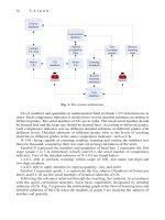
11.5 HMM application: Isolated word recognition
11.6 Sample questions . . . . . . . . . . . . . . . .

.
.
.
.
.
.

.
.
.
.
.
.

.

.
.
.
.
.

.
.
.
.
.
.

.
.
.
.
.
.

.
.
.
.
.
.

.
.
.

.
.
.

.
.
.
.
.
.

.
.
.
.
.
.

.
.
.
.
.
.

.
.
.
.
.

.

.
.
.
.
.
.

.
.
.
.
.
.

.
.
.
.
.
.

.
.
.
.
.
.

.
.
.
.
.
.

.
.
.
.
.
.

.
.
.
.
.
.

.
.
.
.
.
.

.
.

.
.
.
.

.
.
.
.
.
.

161
. 161
. 163
. 167
. 169
. 170
. 171

12 Combining multiple learners
12.1 Why combine many learners
12.2 Ways to achieve diversity . .
12.3 Model combination schemes
12.4 Ensemble learning⋆ . . . . .
12.5 Random forest⋆ . . . . . . .
12.6 Sample questions . . . . . .

.
.

.
.
.
.

.
.
.
.
.
.

.
.
.
.
.
.

.
.
.
.
.
.

.
.
.
.

.
.

.
.
.
.
.
.

.
.
.
.
.
.

.
.
.
.
.
.

.
.
.
.
.
.

.
.
.
.
.
.

.
.
.
.
.
.

.
.
.
.
.
.

.
.
.
.
.
.

.

.
.
.
.
.

.
.
.
.
.
.

.
.
.
.
.
.

.
.
.
.
.
.

.
.
.

.
.
.

.
.
.
.
.
.

.
.
.
.
.
.

.
.
.
.
.
.

173
. 173
. 173
. 174
. 176

. 176
. 178

13 Clustering methods
13.1 Clustering . . . . . . . . . . . . . . . . . . . . . . . .
13.2 k-means clustering . . . . . . . . . . . . . . . . . . .
13.3 Multi-modal distributions . . . . . . . . . . . . . . .
13.4 Mixture of normal distributions . . . . . . . . . . . .
13.5 Mixtures in terms of latent variables . . . . . . . . .
13.6 Expectation-maximisation algorithm . . . . . . . . .
13.7 The EM algorithm for Gaussian mixtures . . . . . .
13.8 Hierarchical clustering . . . . . . . . . . . . . . . . .
13.9 Measures of dissimilarity . . . . . . . . . . . . . . . .
13.10 Algorithm for agglomerative hierarchical clustering
13.11 Algorithm for divisive hierarchical clustering . . . .
13.12 Density-based clustering . . . . . . . . . . . . . . . .
13.13 Sample questions . . . . . . . . . . . . . . . . . . . .

.
.
.
.
.
.
.
.
.
.
.
.

.

.
.
.
.
.
.
.
.
.
.
.
.
.

.
.
.
.
.
.
.
.
.
.
.
.
.

.
.
.
.
.
.
.
.
.
.
.
.
.

.
.
.
.
.
.
.
.
.
.
.
.
.

.
.

.
.
.
.
.
.
.
.
.
.
.

.
.
.
.
.
.
.
.
.
.
.
.
.

.
.
.
.

.
.
.
.
.
.
.
.
.

.
.
.
.
.
.
.
.
.
.
.
.
.

.
.
.
.
.
.

.
.
.
.
.
.
.

.
.
.
.
.
.
.
.
.
.
.
.
.

.
.
.
.
.
.
.
.

.
.
.
.
.

.
.
.
.
.
.
.
.
.
.
.
.
.

.
.
.
.
.
.
.
.
.
.

.
.
.

.
.
.
.
.
.
.
.
.
.
.
.
.

.
.
.
.
.
.
.
.
.
.
.
.

.

.
.
.
.
.
.
.
.
.
.
.
.
.

179
. 179
. 179
. 186
. 186
. 188
. 189
. 190
. 191
. 194
. 196
. 200
. 203
. 204

.
.
.
.
.
.

.
.
.
.
.
.

.
.
.
.
.
.

.
.
.
.
.
.

.

.
.
.
.
.

.
.
.
.
.
.

.
.
.
.
.
.

.
.
.
.
.
.

.
.
.

.
.
.

.
.
.
.
.
.

.
.
.
.
.
.

.
.
.
.
.
.

.
.
.
.
.

.

.
.
.
.
.
.

.
.
.
.
.
.

.
.
.
.
.
.

Bibliography

206

Index

207

List of Figures
1.1
1.2
1.3

1.4
2.1
2.2
2.3
2.4
2.5
2.6
2.7
2.8
3.1
3.2
3.3
3.4
3.5
3.6
4.1
4.2
4.3
4.4
4.5

5.1
5.2

5.3
5.4

6.1

Components of learning process . . . . . . . . . . . . . . . . . . . . . . . . . . . . .
Example for “examples” and “features” collected in a matrix format (data relates
to automobiles and their features) . . . . . . . . . . . . . . . . . . . . . . . . . . . .
Graphical representation of data in Table 1.1. Solid dots represent data in “Pass”
class and hollow dots data in “Fail” class. The class label of the square dot is to be
determined. . . . . . . . . . . . . . . . . . . . . . . . . . . . . . . . . . . . . . . . .
Supervised learning . . . . . . . . . . . . . . . . . . . . . . . . . . . . . . . . . . . .
Data in Table 2.1 with hollow dots representing positive examples and solid dots
representing negative examples . . . . . . . . . . . . . . . . . . . . . . . . . . . . .
An example hypothesis defined by Eq. (2.5) . . . . . . . . . . . . . . . . . . . . . .
Hypothesis h′ is more general than hypothesis h′′ if and only if S ′′ ⊆ S ′ . . . . . .
Values of m which define the version space with data in Table 2.1 and hypothesis
space defined by Eq.(2.4) . . . . . . . . . . . . . . . . . . . . . . . . . . . . . . . . .
Scatter plot of price-power data (hollow circles indicate positive examples and
solid dots indicate negative examples) . . . . . . . . . . . . . . . . . . . . . . . . .
The version space consists of hypotheses corresponding to axis-aligned rectangles
contained in the shaded region . . . . . . . . . . . . . . . . . . . . . . . . . . . . . .
Examples for overfitting and overfitting models . . . . . . . . . . . . . . . . . . . .
Fitting a classification boundary . . . . . . . . . . . . . . . . . . . . . . . . . . . . .
Different forms of the set {x ∈ S ∶ h(x) = 1} for D = {a, b, c} . . . . . . . . . . . .
Geometrical representation of the hypothesis ha,b,c . . . . . . . . . . . . . . . . . .
A hypothesis ha,b,c consistent with the dichotomy defined by the subset {A, C} of
{A, B, C} . . . . . . . . . . . . . . . . . . . . . . . . . . . . . . . . . . . . . . . . .
There is no hypothesis ha,b,c consistent with the dichotomy defined by the subset
{A, C} of {A, B, C, D} . . . . . . . . . . . . . . . . . . . . . . . . . . . . . . . . .

An axis-aligned rectangle in the Euclidean plane . . . . . . . . . . . . . . . . . . .
Axis-aligned rectangle which gives the tightest fit to the positive examples . . . .

.

2

.

5

. 7
. 12

. 16
. 17
. 18
. 19
. 20
. 20
. 24
. 25
. 28
. 30
. 30
. 30
. 32
. 33

Principal components . . . . . . . . . . . . . . . . . . . . . . . . . . . . . . . . . . .

Scatter plot of data in Table 4.2 . . . . . . . . . . . . . . . . . . . . . . . . . . . . .
Coordinate system for principal components . . . . . . . . . . . . . . . . . . . . . .
Projections of data points on the axis of the first principal component . . . . . . .
Geometrical representation of one-dimensional approximation to the data in Table
4.2 . . . . . . . . . . . . . . . . . . . . . . . . . . . . . . . . . . . . . . . . . . . . .

.
.
.
.

39
43
45
46

One iteration in a 5-fold cross-validation . . . . . . . . . . . . . . . . . . . . . . . .
The ROC space and some special points in the space . . . . . . . . . . . . . . . . .
ROC curves of three different classifiers A, B, C . . . . . . . . . . . . . . . . . . .
ROC curve of data in Table 5.3 showing the points closest to the perfect prediction
point (0, 1) . . . . . . . . . . . . . . . . . . . . . . . . . . . . . . . . . . . . . . . .

. 50
. 56
. 57

. 46

. 58

Events A, B, C which are not mutually independent: Eqs.(6.1)–(6.3) are satisfied,
but Eq.(6.4) is not satisfied. . . . . . . . . . . . . . . . . . . . . . . . . . . . . . . . . 62
xi


LIST OF FIGURES

xii

6.3

Events A, B, C which are not mutually independent: Eq.(6.4) is satisfied but Eqs.(6.1)–
(6.2) are not satisfied. . . . . . . . . . . . . . . . . . . . . . . . . . . . . . . . . . . . . 62
Discretization of numeric data: Example . . . . . . . . . . . . . . . . . . . . . . . . . 68

7.1
7.2
7.3
7.4

Errors in observed values . . . . . . . . . . . .
Regression model for Table 7.2 . . . . . . . .
Plot of quadratic polynomial model . . . . . .
The regression plane for the data in Table 7.4

8.1
8.2
8.3
8.4
8.5

8.6
8.7
8.8
8.9
8.10
8.11
8.12
8.13
8.14

Example for a decision tree . . . . . . . . . . . . . . . . . . . . . . . . . . . . . . . . 83
The graph-theoretical representation of the decision tree in Figure 8.6 . . . . . . . . 84
Classification tree . . . . . . . . . . . . . . . . . . . . . . . . . . . . . . . . . . . . . . 85
Classification tree . . . . . . . . . . . . . . . . . . . . . . . . . . . . . . . . . . . . . . 86
Classification tree . . . . . . . . . . . . . . . . . . . . . . . . . . . . . . . . . . . . . . 88
Plot of p vs. Entropy . . . . . . . . . . . . . . . . . . . . . . . . . . . . . . . . . . . . 90
Root node of the decision tree for data in Table 8.9 . . . . . . . . . . . . . . . . . . . 97
Decision tree for data in Table 8.9, after selecting the branching feature at root node 99
Decision tree for data in Table 8.9, after selecting the branching feature at Node 1 . 100
Decision tree for data in Table 8.9 . . . . . . . . . . . . . . . . . . . . . . . . . . . . . 101
Part of a regression tree for Table 8.11 . . . . . . . . . . . . . . . . . . . . . . . . . . 102
Part of regression tree for Table 8.11 . . . . . . . . . . . . . . . . . . . . . . . . . . . 102
A regression tree for Table 8.11 . . . . . . . . . . . . . . . . . . . . . . . . . . . . . . 103
Impact of overfitting in decision tree learning . . . . . . . . . . . . . . . . . . . . . . 107

9.1
9.2
9.3
9.4
9.5

9.6
9.7
9.8
9.9
9.10
9.11
9.12
9.13
9.14
9.15
9.16
9.17
9.18
9.19
9.20
9.21
9.22
9.23

Anatomy of a neuron . . . . . . . . . . . . . . . . . . . . . . . . . . . . . . . . .
Flow of signals in a biological neuron . . . . . . . . . . . . . . . . . . . . . . .
Schematic representation of an artificial neuron . . . . . . . . . . . . . . . . . .
Simplified representation of an artificial neuron . . . . . . . . . . . . . . . . . .
Threshold activation function . . . . . . . . . . . . . . . . . . . . . . . . . . . .
Unit step activation function . . . . . . . . . . . . . . . . . . . . . . . . . . . . .
The sigmoid activation function . . . . . . . . . . . . . . . . . . . . . . . . . . .
Linear activation function . . . . . . . . . . . . . . . . . . . . . . . . . . . . . .
Piecewise linear activation function . . . . . . . . . . . . . . . . . . . . . . . . .
Gaussian activation function . . . . . . . . . . . . . . . . . . . . . . . . . . . . .
Hyperbolic tangent activation function . . . . . . . . . . . . . . . . . . . . . . .

Schematic representation of a perceptrn . . . . . . . . . . . . . . . . . . . . . .
Representation of x1 AND x2 by a perceptron . . . . . . . . . . . . . . . . . . .
An ANN with only one layer . . . . . . . . . . . . . . . . . . . . . . . . . . . .
An ANN with two layers . . . . . . . . . . . . . . . . . . . . . . . . . . . . . . .
Examples of different topologies of networks . . . . . . . . . . . . . . . . . . .
A simplified model of the error surface showing the direction of gradient . . .
ANN for illustrating backpropagation algorithm . . . . . . . . . . . . . . . . . .
ANN for illustrating backpropagation algorithm with initial values for weights
Notations of backpropagation algorithm . . . . . . . . . . . . . . . . . . . . . .
Notations of backpropagation algorithm: The i-th node in layer j . . . . . . . .
A shallow neural network . . . . . . . . . . . . . . . . . . . . . . . . . . . . . .
A deep neural network with three hidden layers . . . . . . . . . . . . . . . . . .

.
.
.
.
.
.
.
.
.
.
.
.
.
.
.
.
.

.
.
.
.
.
.

. 111
. 112
. 112
. 113
. 114
. 114
. 114
. 115
. 115
. 115
. 116
. 116
. 117
. 120
. 121
. 122
. 123
. 124
. 124
. 128
. 128
. 130
. 130

10.1

Scatter plot of data in Table 10.1 (filled circles represent “yes” and unfilled circles
“no”) . . . . . . . . . . . . . . . . . . . . . . . . . . . . . . . . . . . . . . . . . . . .
Scatter plot of data in Table 10.1 with a separating line . . . . . . . . . . . . . . . .
Two separating lines for the data in Table 10.1 . . . . . . . . . . . . . . . . . . . . .
Shortest perpendicular distance of a separating line from data points . . . . . . . .
Maximum margin line for data in Table 10.1 . . . . . . . . . . . . . . . . . . . . . .
Support vectors for data in Table 10.1 . . . . . . . . . . . . . . . . . . . . . . . . .

. 134
. 135
. 135
. 136
. 136
. 137

6.2

10.2
10.3
10.4
10.5
10.6

.
.
.
.

.
.
.
.

.
.
.
.

.
.
.
.

.
.
.
.

.
.
.
.

.
.
.
.

.
.
.
.

.
.
.
.

.
.
.
.

.
.
.
.

.
.
.
.

.
.
.
.

.
.
.
.

.
.
.
.

.
.
.
.

.
.
.
.

.
.
.
.

.
.
.
.

.
.
.
.

.
.
.
.
.
.
.
.
.
.
.
.
.
.
.
.
.
.
.
.
.
.
.

.
.
.
.

.
.
.
.

74
76
78
80


LIST OF FIGURES
10.7
10.8
10.9
10.10
10.11
10.12
10.13
10.14
10.15
10.16
10.17
11.1
11.2

11.3

xiii

Boundaries of “street” of maximum width separating “yes” points and “no” points
in Table 10.1 . . . . . . . . . . . . . . . . . . . . . . . . . . . . . . . . . . . . . . . .
Plot of the maximum margin line of data in Table 10.1 produced by the R programming language . . . . . . . . . . . . . . . . . . . . . . . . . . . . . . . . . . . . . .
Half planes defined by a line . . . . . . . . . . . . . . . . . . . . . . . . . . . . . . .
Perpendicular distance of a point from a plane . . . . . . . . . . . . . . . . . . . . .
Scatterplot of data in Table 10.2 . . . . . . . . . . . . . . . . . . . . . . . . . . . . .
Maximal separating hyperplane, margin and support vectors . . . . . . . . . . . . .
Maximal margin hyperplane of a 2-sample set in 2-dimensional space . . . . . . .
Maximal margin hyperplane of a 3-sample set in 2-dimensional space . . . . . . .
Soft margin hyperplanes . . . . . . . . . . . . . . . . . . . . . . . . . . . . . . . . .
One-against all . . . . . . . . . . . . . . . . . . . . . . . . . . . . . . . . . . . . . .
One-against-one . . . . . . . . . . . . . . . . . . . . . . . . . . . . . . . . . . . . . .

. 138
. 142
. 143
. 145
. 146
. 147
. 147
. 155
. 158
. 159

11.4

A state diagram showing state transition probabilities .
A two-coin model of an HMM . . . . . . . . . . . . . .
An N -state urn and ball model which illustrates the
symbol HMM . . . . . . . . . . . . . . . . . . . . . . .
Block diagram of an isolated word HMM recogniser .

12.1

Example of random forest with majority voting . . . . . . . . . . . . . . . . . . . . . 177

13.1
13.2
13.3
13.4
13.5
13.6

Scatter diagram of data in Table 13.1 . . . . . . . . . . . . . . . . . . . . . . . . . .
Initial choice of cluster centres and the resulting clusters . . . . . . . . . . . . . . .
Cluster centres after first iteration and the corresponding clusters . . . . . . . . . .
New cluster centres and the corresponding clusters . . . . . . . . . . . . . . . . . .
Probability distributions . . . . . . . . . . . . . . . . . . . . . . . . . . . . . . . . .
Graph of pdf defined by Eq.(13.9) superimposed on the histogram of the data in
Table 13.3 . . . . . . . . . . . . . . . . . . . . . . . . . . . . . . . . . . . . . . . . .
A dendrogram of the dataset {a, b, c, d, e} . . . . . . . . . . . . . . . . . . . . . . .
Different ways of drawing dendrogram . . . . . . . . . . . . . . . . . . . . . . . . .
A dendrogram of the dataset {a, b, c, d, e} showing the distances (heights) of the
clusters at different levels . . . . . . . . . . . . . . . . . . . . . . . . . . . . . . . .
Hierarchical clustering using agglomerative method . . . . . . . . . . . . . . . . .
Hierarchical clustering using divisive method . . . . . . . . . . . . . . . . . . . . .

Length of the solid line “ae” is max{d(x, y) ∶ x ∈ A, y ∈ B} . . . . . . . . . . . . .
Length of the solid line “bc” is min{d(x, y) ∶ x ∈ A, y ∈ B} . . . . . . . . . . . . .
Dendrogram for the data given in Table 13.4 (complete linkage clustering) . . . .
Dendrogram for the data given in Table 13.4 (single linkage clustering) . . . . . .
Dx = (average of dashed lines) − (average of solid lines) . . . . . . . . . . . . . . .
Clusters of points and noise points not belonging to any of those clusters . . . . .
With m0 = 4: (a) p a point of high density (b) p a core point (c) p a border point
(d) r a noise point . . . . . . . . . . . . . . . . . . . . . . . . . . . . . . . . . . . . .
With m0 = 4: (a) q is directly density-reachable from p (b) q is indirectly densityreachable from p . . . . . . . . . . . . . . . . . . . . . . . . . . . . . . . . . . . . .

13.7
13.8
13.9
13.10
13.11
13.12
13.13
13.14
13.15
13.16
13.17
13.18
13.19

. . . . . . . . . . . . . . . .
. . . . . . . . . . . . . . . .
general case of a discrete
. . . . . . . . . . . . . . . .
. . . . . . . . . . . . . . . .

. 137

. 162
. 167
. 168
. 171

. 180
. 181
. 182
. 183
. 186
. 188
. 192
. 192
. 192
. 193
. 195
. 196
. 196
. 199
. 200
. 201
. 203
. 203
. 204


Chapter 1

Introduction to machine learning
In this chapter, we consider different definitions of the term “machine learning” and explain what
is meant by “learning” in the context of machine learning. We also discuss the various components
of the machine learning process. There are also brief discussions about different types learning like
supervised learning, unsupervised learning and reinforcement learning.

1.1
1.1.1

Introduction
Definition of machine learning

Arthur Samuel, an early American leader in the field of computer gaming and artificial intelligence,
coined the term “Machine Learning” in 1959 while at IBM. He defined machine learning as “the field
of study that gives computers the ability to learn without being explicitly programmed.” However,
there is no universally accepted definition for machine learning. Different authors define the term
differently. We give below two more definitions.
1. Machine learning is programming computers to optimize a performance criterion using example data or past experience. We have a model defined up to some parameters, and learning is
the execution of a computer program to optimize the parameters of the model using the training data or past experience. The model may be predictive to make predictions in the future, or
descriptive to gain knowledge from data, or both (see [2] p.3).
2. The field of study known as machine learning is concerned with the question of how to construct computer programs that automatically improve with experience (see [4], Preface.).
Remarks
In the above definitions we have used the term “model” and we will be using this term at several
contexts later in this book. It appears that there is no universally accepted one sentence definition
of this term. Loosely, it may be understood as some mathematical expression or equation, or some
mathematical structures such as graphs and trees, or a division of sets into disjoint subsets, or a set
of logical “if . . . then . . . else . . .” rules, or some such thing. It may be noted that this is not an
exhaustive list.

1.1.2

Definition of learning

Definition
A computer program is said to learn from experience E with respect to some class of tasks T and
performance measure P , if its performance at tasks T , as measured by P , improves with experience
E.
1


CHAPTER 1. INTRODUCTION TO MACHINE LEARNING

2

Examples
i) Handwriting recognition learning problem
• Task T : Recognising and classifying handwritten words within images
• Performance P : Percent of words correctly classified
• Training experience E: A dataset of handwritten words with given classifications
ii) A robot driving learning problem
• Task T : Driving on highways using vision sensors
• Performance measure P : Average distance traveled before an error
• training experience: A sequence of images and steering commands recorded while
observing a human driver
iii) A chess learning problem
• Task T : Playing chess
• Performance measure P : Percent of games won against opponents
• Training experience E: Playing practice games against itself
Definition
A computer program which learns from experience is called a machine learning program or simply

a learning program. Such a program is sometimes also referred to as a learner.

1.2
1.2.1

How machines learn
Basic components of learning process

The learning process, whether by a human or a machine, can be divided into four components,
namely, data storage, abstraction, generalization and evaluation. Figure 1.1 illustrates the various
components and the steps involved in the learning process.
Data storage
Abstraction
Generalization
Evaluation

Data

Concepts

Inferences

Figure 1.1: Components of learning process
1. Data storage
Facilities for storing and retrieving huge amounts of data are an important component of
the learning process. Humans and computers alike utilize data storage as a foundation for
advanced reasoning.
• In a human being, the data is stored in the brain and data is retrieved using electrochemical signals.
• Computers use hard disk drives, flash memory, random access memory and similar devices to store data and use cables and other technology to retrieve data.

CHAPTER 1. INTRODUCTION TO MACHINE LEARNING

3

2. Abstraction
The second component of the learning process is known as abstraction.
Abstraction is the process of extracting knowledge about stored data. This involves creating
general concepts about the data as a whole. The creation of knowledge involves application
of known models and creation of new models.
The process of fitting a model to a dataset is known as training. When the model has been
trained, the data is transformed into an abstract form that summarizes the original information.
3. Generalization
The third component of the learning process is known as generalisation.
The term generalization describes the process of turning the knowledge about stored data into
a form that can be utilized for future action. These actions are to be carried out on tasks that
are similar, but not identical, to those what have been seen before. In generalization, the goal
is to discover those properties of the data that will be most relevant to future tasks.
4. Evaluation
Evaluation is the last component of the learning process.
It is the process of giving feedback to the user to measure the utility of the learned knowledge.
This feedback is then utilised to effect improvements in the whole learning process.

1.3

Applications of machine learning

Application of machine learning methods to large databases is called data mining. In data mining, a
large volume of data is processed to construct a simple model with valuable use, for example, having
high predictive accuracy.

The following is a list of some of the typical applications of machine learning.
1. In retail business, machine learning is used to study consumer behaviour.
2. In finance, banks analyze their past data to build models to use in credit applications, fraud
detection, and the stock market.
3. In manufacturing, learning models are used for optimization, control, and troubleshooting.
4. In medicine, learning programs are used for medical diagnosis.
5. In telecommunications, call patterns are analyzed for network optimization and maximizing
the quality of service.
6. In science, large amounts of data in physics, astronomy, and biology can only be analyzed fast
enough by computers. The World Wide Web is huge; it is constantly growing and searching
for relevant information cannot be done manually.
7. In artificial intelligence, it is used to teach a system to learn and adapt to changes so that the
system designer need not foresee and provide solutions for all possible situations.
8. It is used to find solutions to many problems in vision, speech recognition, and robotics.
9. Machine learning methods are applied in the design of computer-controlled vehicles to steer
correctly when driving on a variety of roads.
10. Machine learning methods have been used to develop programmes for playing games such as
chess, backgammon and Go.


CHAPTER 1. INTRODUCTION TO MACHINE LEARNING

1.4

4

Understanding data

Since an important component of the machine learning process is data storage, we briefly consider
in this section the different types and forms of data that are encountered in the machine learning

process.

1.4.1

Unit of observation

By a unit of observation we mean the smallest entity with measured properties of interest for a study.
Examples
• A person, an object or a thing
• A time point
• A geographic region
• A measurement
Sometimes, units of observation are combined to form units such as person-years.

1.4.2

Examples and features

Datasets that store the units of observation and their properties can be imagined as collections of
data consisting of the following:
• Examples
An “example” is an instance of the unit of observation for which properties have been recorded.
An “example” is also referred to as an “instance”, or “case” or “record.” (It may be noted that
the word “example” has been used here in a technical sense.)
• Features
A “feature” is a recorded property or a characteristic of examples. It is also referred to as
“attribute”, or “variable” or “feature.”
Examples for “examples” and “features”
1. Cancer detection
Consider the problem of developing an algorithm for detecting cancer. In this study we note

the following.
(a) The units of observation are the patients.
(b) The examples are members of a sample of cancer patients.
(c) The following attributes of the patients may be chosen as the features:
•
•
•
•

gender
age
blood pressure
the findings of the pathology report after a biopsy

2. Pet selection
Suppose we want to predict the type of pet a person will choose.
(a) The units are the persons.
(b) The examples are members of a sample of persons who own pets.


CHAPTER 1. INTRODUCTION TO MACHINE LEARNING

5

Figure 1.2: Example for “examples” and “features” collected in a matrix format (data relates to
automobiles and their features)

(c) The features might include age, home region, family income, etc. of persons who own
pets.
3. Spam e-mail

Let it be required to build a learning algorithm to identify spam e-mail.
(a) The unit of observation could be an e-mail messages.
(b) The examples would be specific messages.
(c) The features might consist of the words used in the messages.
Examples and features are generally collected in a “matrix format”. Fig. 1.2 shows such a data
set.

1.4.3

Different forms of data

1. Numeric data
If a feature represents a characteristic measured in numbers, it is called a numeric feature.
2. Categorical or nominal
A categorical feature is an attribute that can take on one of a limited, and usually fixed, number
of possible values on the basis of some qualitative property. A categorical feature is also called
a nominal feature.
3. Ordinal data
This denotes a nominal variable with categories falling in an ordered list. Examples include
clothing sizes such as small, medium, and large, or a measurement of customer satisfaction
on a scale from “not at all happy” to “very happy.”
Examples
In the data given in Fig.1.2, the features “year”, “price” and “mileage” are numeric and the features
“model”, “color” and “transmission” are categorical.


CHAPTER 1. INTRODUCTION TO MACHINE LEARNING

1.5
1.5.1

6

General classes of machine learning problems
Learning associations

1. Association rule learning
Association rule learning is a machine learning method for discovering interesting relations, called
“association rules”, between variables in large databases using some measures of “interestingness”.
2. Example
Consider a supermarket chain. The management of the chain is interested in knowing whether
there are any patterns in the purchases of products by customers like the following:
“If a customer buys onions and potatoes together, then he/she is likely to also buy
hamburger.”
From the standpoint of customer behaviour, this defines an association between the set of
products {onion, potato} and the set {burger}. This association is represented in the form of
a rule as follows:
{onion, potato} ⇒ {burger}
The measure of how likely a customer, who has bought onion and potato, to buy burger also
is given by the conditional probability
P ({onion, potato}∣{burger}).
If this conditional probability is 0.8, then the rule may be stated more precisely as follows:
“80% of customers who buy onion and potato also buy burger.”
3. How association rules are made use of
Consider an association rule of the form

X ⇒ Y,

that is, if people buy X then they are also likely to buy Y .
Suppose there is a customer who buys X and does not buy Y . Then that customer is a potential

Y customer. Once we find such customers, we can target them for cross-selling. A knowledge of
such rules can be used for promotional pricing or product placements.
4. General case
In finding an association rule X ⇒ Y , we are interested in learning a conditional probability of
the form P (Y ∣X) where Y is the product the customer may buy and X is the product or the set of
products the customer has already purchased.
If we may want to make a distinction among customers, we may estimate P (Y ∣X, D) where
D is a set of customer attributes, like gender, age, marital status, and so on, assuming that we have
access to this information.
5. Algorithms
There are several algorithms for generating association rules. Some of the well-known algorithms
are listed below:
a) Apriori algorithm
b) Eclat algorithm
c) FP-Growth Algorithm (FP stands for Frequency Pattern)


CHAPTER 1. INTRODUCTION TO MACHINE LEARNING

1.5.2

7

Classification

1. Definition
In machine learning, classification is the problem of identifying to which of a set of categories a
new observation belongs, on the basis of a training set of data containing observations (or instances)
whose category membership is known.
2. Example

Consider the following data:
Score1
Score2
Result

29
43
Pass

22
29
Fail

10
47
Fail

31
55
Pass

17
18
Fail

33
54
Pass

32

40
Pass

20
41
Pass

Table 1.1: Example data for a classification problem

Data in Table 1.1 is the training set of data. There are two attributes “Score1” and “Score2”. The
class label is called “Result”. The class label has two possible values “Pass” and “Fail”. The data
can be divided into two categories or classes: The set of data for which the class label is “Pass” and
the set of data for which the class label is“Fail”.
Let us assume that we have no knowledge about the data other than what is given in the table.
Now, the problem can be posed as follows: If we have some new data, say “Score1 = 25” and
“Score2 = 36”, what value should be assigned to “Result” corresponding to the new data; in other
words, to which of the two categories or classes the new observation should be assigned? See Figure
1.3 for a graphical representation of the problem.
Score2
60
50
40
?

30
20
10
0

10

20

30

Score1
40

Figure 1.3: Graphical representation of data in Table 1.1. Solid dots represent data in “Pass” class
and hollow dots data in “Fail” class. The class label of the square dot is to be determined.

To answer this question, using the given data alone we need to find the rule, or the formula, or
the method that has been used in assigning the values to the class label “Result”. The problem of
finding this rule or formula or the method is the classification problem. In general, even the general
form of the rule or function or method will not be known. So several different rules, etc. may have
to be tested to obtain the correct rule or function or method.


CHAPTER 1. INTRODUCTION TO MACHINE LEARNING

8

3. Real life examples
i) Optical character recognition
Optical character recognition problem, which is the problem of recognizing character codes
from their images, is an example of classification problem. This is an example where there
are multiple classes, as many as there are characters we would like to recognize. Especially
interesting is the case when the characters are handwritten. People have different handwriting styles; characters may be written small or large, slanted, with a pen or pencil, and there
are many possible images corresponding to the same character.
ii) Face recognition

In the case of face recognition, the input is an image, the classes are people to be recognized,
and the learning program should learn to associate the face images to identities. This problem is more difficult than optical character recognition because there are more classes, input
image is larger, and a face is three-dimensional and differences in pose and lighting cause
significant changes in the image.
iii) Speech recognition
In speech recognition, the input is acoustic and the classes are words that can be uttered.
iv) Medical diagnosis
In medical diagnosis, the inputs are the relevant information we have about the patient and
the classes are the illnesses. The inputs contain the patient’s age, gender, past medical
history, and current symptoms. Some tests may not have been applied to the patient, and
thus these inputs would be missing.
v) Knowledge extraction
Classification rules can also be used for knowledge extraction. The rule is a simple model
that explains the data, and looking at this model we have an explanation about the process
underlying the data.
vi) Compression
Classification rules can be used for compression. By fitting a rule to the data, we get an
explanation that is simpler than the data, requiring less memory to store and less computation
to process.
vii) More examples
Here are some further examples of classification problems.
(a) An emergency room in a hospital measures 17 variables like blood pressure, age, etc.
of newly admitted patients. A decision has to be made whether to put the patient in an
ICU. Due to the high cost of ICU, only patients who may survive a month or more are
given higher priority. Such patients are labeled as “low-risk patients” and others are
labeled “high-risk patients”. The problem is to device a rule to classify a patient as a
“low-risk patient” or a “high-risk patient”.
(b) A credit card company receives hundreds of thousands of applications for new cards.
The applications contain information regarding several attributes like annual salary,
age, etc. The problem is to devise a rule to classify the applicants to those who are

credit-worthy, who are not credit-worthy or to those who require further analysis.
(c) Astronomers have been cataloguing distant objects in the sky using digital images created using special devices. The objects are to be labeled as star, galaxy, nebula, etc.
The data is highly noisy and are very faint. The problem is to device a rule using which
a distant object can be correctly labeled.


CHAPTER 1. INTRODUCTION TO MACHINE LEARNING

9

4. Discriminant
A discriminant of a classification problem is a rule or a function that is used to assign labels to new
observations.
Examples
i) Consider the data given in Table 1.1 and the associated classification problem. We may
consider the following rules for the classification of the new data:
IF Score1 + Score2 ≥ 60, THEN “Pass” ELSE “Fail”.
IF Score1 ≥ 20 AND Score2 ≥ 40 THEN “Pass” ELSE “Fail”.
Or, we may consider the following rules with unspecified values for M, m1 , m2 and then by
some method estimate their values.
IF Score1 + Score2 ≥ M , THEN “Pass” ELSE “Fail”.
IF Score1 ≥ m1 AND Score2 ≥ m2 THEN “Pass” ELSE “Fail”.
ii) Consider a finance company which lends money to customers. Before lending money, the
company would like to assess the risk associated with the loan. For simplicity, let us assume
that the company assesses the risk based on two variables, namely, the annual income and
the annual savings of the customers.
Let x1 be the annual income and x2 be the annual savings of a customer.
• After using the past data, a rule of the following form with suitable values for θ1 and
θ2 may be formulated:
IF x1 > θ1 AND x2 > θ2 THEN “low-risk” ELSE “high-risk”.

This rule is an example of a discriminant.
• Based on the past data, a rule of the following form may also be formulated:
IF x2 − 0.2x1 > 0 THEN “low-risk” ELSE “high-risk”.
In this case the rule may be thought of as the discriminant. The function f (x1 , x2 ) =
x2 − 0, 2x1 can also be considered as the discriminant.
5. Algorithms
There are several machine learning algorithms for classification. The following are some of the
well-known algorithms.
a) Logistic regression
b) Naive Bayes algorithm
c) k-NN algorithm
d) Decision tree algorithm
e) Support vector machine algorithm
f) Random forest algorithm


CHAPTER 1. INTRODUCTION TO MACHINE LEARNING

10

Remarks
• A classification problem requires that examples be classified into one of two or more classes.
• A classification can have real-valued or discrete input variables.
• A problem with two classes is often called a two-class or binary classification problem.
• A problem with more than two classes is often called a multi-class classification problem.
• A problem where an example is assigned multiple classes is called a multi-label classification
problem.

1.5.3

Regression

1. Definition
In machine learning, a regression problem is the problem of predicting the value of a numeric variable based on observed values of the variable. The value of the output variable may be a number,
such as an integer or a floating point value. These are often quantities, such as amounts and sizes.
The input variables may be discrete or real-valued.
2. Example
Consider the data on car prices given in Table 1.2.
Price
(US$)
13500
13750
13950
14950
13750
12950
16900
18600
21500
12950

Age
(years)
23
23
24
26
30
32
27

30
27
23

Distance
(KM)
46986
72937
41711
48000
38500
61000
94612
75889
19700
71138

Weight
(pounds)
1165
1165
1165
1165
1170
1170
1245
1245
1185
1105

Table 1.2: Prices of used cars: example data for regression
Suppose we are required to estimate the price of a car aged 25 years with distance 53240 KM
and weight 1200 pounds. This is an example of a regression problem beause we have to predict the
value of the numeric variable “Price”.
3. General approach
Let x denote the set of input variables and y the output variable. In machine learning, the general
approach to regression is to assume a model, that is, some mathematical relation between x and y,
involving some parameters say, θ, in the following form:
y = f (x, θ)
The function f (x, θ) is called the regression function. The machine learning algorithm optimizes
the parameters in the set θ such that the approximation error is minimized; that is, the estimates
of the values of the dependent variable y are as close as possible to the correct values given in the
training set.