Báo cáo khoa học: "A Nonparametric Bayesian Approach to Acoustic Model Discovery" docx

Proceedings of the 50th Annual Meeting of the Association for Computational Linguistics, pages 40–49,
Jeju, Republic of Korea, 8-14 July 2012.
c
2012 Association for Computational Linguistics
A Nonparametric Bayesian Approach to Acoustic Model Discovery
Chia-ying Lee and James Glass
Computer Science and Artificial Intelligence Laboratory
Massachusetts Institute of Technology
Cambridge, MA 02139, USA
{chiaying,jrg}@csail.mit.edu
Abstract
We investigate the problem of acoustic mod-
eling in which prior language-specific knowl-
edge and transcribed data are unavailable. We
present an unsupervised model that simultane-
ously segments the speech, discovers a proper
set of sub-word units (e.g., phones) and learns
a Hidden Markov Model (HMM) for each in-
duced acoustic unit. Our approach is formu-
lated as a Dirichlet process mixture model in
which each mixture is an HMM that repre-
sents a sub-word unit. We apply our model
to the TIMIT corpus, and the results demon-
strate that our model discovers sub-word units
that are highly correlated with English phones
and also produces better segmentation than the
state-of-the-art unsupervised baseline. We test
the quality of the learned acoustic models on a
spoken term detection task. Compared to the
baselines, our model improves the relative pre-
cision of top hits by at least 22.1% and outper-

forms a language-mismatched acoustic model.
1 Introduction
Acoustic models are an indispensable component
of speech recognizers. However, the standard pro-
cess of training acoustic models is expensive, and
requires not only language-specific knowledge, e.g.,
the phone set of the language, a pronunciation dic-
tionary, but also a large amount of transcribed data.
Unfortunately, these necessary data are only avail-
able for a very small number of languages in the
world. Therefore, a procedure for training acous-
tic models without annotated data would not only
be a breakthrough from the traditional approach, but
would also allow us to build speech recognizers for
any language efficiently.
In this paper, we investigate the problem of unsu-
pervised acoustic modeling with only spoken utter-
ances as training data. As suggested in Garcia and
Gish (2006), unsupervised acoustic modeling can
be broken down to three sub-tasks: segmentation,
clustering segments, and modeling the sound pattern
of each cluster. In previous work, the three sub-
problems were often approached sequentially and
independently in which initial steps are not related to
later ones (Lee et al., 1988; Garcia and Gish, 2006;
Chan and Lee, 2011). For example, the speech data
was usually segmented regardless of the clustering
results and the learned acoustic models.
In contrast to the previous methods, we approach
the problem by modeling the three sub-problems as

well as the unknown set of sub-word units as la-
tent variables in one nonparametric Bayesian model.
More specifically, we formulate a Dirichlet pro-
cess mixture model where each mixture is a Hid-
den Markov Model (HMM) used to model a sub-
word unit and to generate observed segments of that
unit. Our model seeks the set of sub-word units,
segmentation, clustering and HMMs that best repre-
sent the observed data through an iterative inference
process. We implement the inference process using
Gibbs sampling.
We test the effectiveness of our model on the
TIMIT database (Garofolo et al., 1993). Our model
shows its ability to discover sub-word units that are
highly correlated with standard English phones and
to capture acoustic context information. For the seg-
mentation task, our model outperforms the state-of-
40
the-art unsupervised method and improves the rel-
ative F-score by 18.8 points (Dusan and Rabiner,
2006). Finally, we test the quality of the learned
acoustic models through a keyword spotting task.
Compared to the state-of-the-art unsupervised meth-
ods (Zhang and Glass, 2009; Zhang et al., 2012),
our model yields a relative improvement in precision
of top hits by at least 22.1% with only some degra-
dation in equal error rate (EER), and outperforms
a language-mismatched acoustic model trained with
supervised data.
2 Related Work

Unsupervised Sub-word Modeling We follow
the general guideline used in (Lee et al., 1988; Gar-
cia and Gish, 2006; Chan and Lee, 2011) and ap-
proach the problem of unsupervised acoustic mod-
eling by solving three sub-problems of the task:
segmentation, clustering and modeling each cluster.
The key difference, however, is that our model does
not assume independence among the three aspects of
the problem, which allows our model to refine its so-
lution to one sub-problem by exploiting what it has
learned about other parts of the problem. Second,
unlike (Lee et al., 1988; Garcia and Gish, 2006) in
which the number of sub-word units to be learned is
assumed to be known, our model learns the proper
size from the training data directly.
Instead of segmenting utterances, the authors
of (Varadarajan et al., 2008) trained a single state
HMM using all data at first, and then iteratively
split the HMM states based on objective functions.
This method achieved high performance in a phone
recognition task using a label-to-phone transducer
trained from some transcriptions. However, the per-
formance seemed to rely on the quality of the trans-
ducer. For our work, we assume no transcriptions
are available and measure the quality of the learned
acoustic units via a spoken query detection task as
in Jansen and Church (2011).
Jansen and Church (2011) approached the task of
unsupervised acoustic modeling by first discovering
repetitive patterns in the data, and then learned a

whole-word HMM for each found pattern, where the
state number of each HMM depends on the average
length of the pattern. The states of the whole-word
HMMs were then collapsed and used to represent
acoustic units. Instead of discovering repetitive pat-
terns first, our model is able to learn from any given
data.
Unsupervised Speech Segmentation One goal
of our model is to segment speech data into
small sub-word (e.g., phone) segments. Most un-
supervised speech segmentation methods rely on
acoustic change for hypothesizing phone bound-
aries (Scharenborg et al., 2010; Qiao et al., 2008;
Dusan and Rabiner, 2006; Estevan et al., 2007).
Even though the overall approaches differ, these al-
gorithms are all one-stage and bottom-up segmenta-
tion methods (Scharenborg et al., 2010). Our model
does not make a single one-stage decision; instead, it
infers the segmentation through an iterative process
and exploits the learned sub-word models to guide
its hypotheses on phone boundaries.
Bayesian Model for Segmentation Our model is
inspired by previous applications of nonparametric
Bayesian models to segmentation problems in NLP
and speaker diarization (Goldwater, 2009; Fox et al.,
2011); particularly, we adapt the inference method
used in (Goldwater, 2009) to our segmentation task.
Our problem is, in principle, similar to the word seg-
mentation problem discussed in (Goldwater, 2009).
The main difference, however, is that our model

is under the continuous real value domain, and the
problem of (Goldwater, 2009) is under the discrete
symbolic domain. For the domain our problem is ap-
plied to, our model has to include more latent vari-
ables and is more complex.
3 Problem Formulation
The goal of our model, given a set of spoken utter-
ances, is to jointly learn the following:
• Segmentation: To find the phonetic boundaries
within each utterance.
• Nonparametric clustering: To find a proper set
of clusters and group acoustically similar seg-
ments into the same cluster.
• Sub-word modeling: To learn a HMM to model
each sub-word acoustic unit.
We model the three sub-tasks as latent variables
in our approach. In this section, we describe the ob-
served data, latent variables, and auxiliary variables
41
€
x
2
i
€
x
3
i
€
x
4

i
€
x
5
i
€
x
6
i
€
x
7
i
€
x
8
i
€
x
9
i
€
x
10
i
€
x
11
i
€

x
1
i
b a
n a
n a
€
(x
t
i
)
€
(t )
1
2
3 4 5 6 7 8 9 10 11
€
(b
t
i
)
€
(g
q
i
)
€
g
0
i

€
g
1
i
€
g
2
i
€
g
3
i
€
g
4
i
€
g
5
i
€
g
6
i
€
( p
j,k
i
)
€

p
1,1
i
€
p
2,4
i
€
p
5,6
i
€
p
7,8
i
€
p
9,9
i
€
p
10,11
i
€
(c
j,k
i
)
€
c

1,1
i
€
c
2,4
i
€
c
5,6
i
€
c
7,8
i
€
c
9,9
i
€
c
10,11
i
€
(
θ
c
)
€
θ
1

€
θ
2
€
θ
3
€
θ
4
€
θ
3
€
θ
2
€
(s
t
i
)
1
1
2 3 1 3 1 3 1 1 3
Frame index
Speech feature
Boundary variable
Boundary index
Segment
Cluster label
HMM

Hidden state
[b] [ax]
[n]
[ae]
[n] [ax]
Pronunciation
1
0
0 1 0 1 0 1 1 0 1
Duration
€
(d
j,k
i
)
1
3 2 2 1 2
1
1
6 8 3 7 5 2 8 2 8
Mixture ID
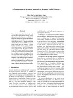
Figure 1: An example of the observed data and hidden
variables of the problem for the word banana. See Sec-
tion 3 for a detailed explanation.
of the problem and show an example in Fig. 1. In
the next section, we show the generative process our
model uses to generate the observed data.
Speech Feature (x
i
t

) The only observed data for
our problem are a set of spoken utterances, which are
converted to a series of 25 ms 13-dimensional Mel-
Frequency Cepstral Coefficients (MFCCs) (Davis
and Mermelstein, 1980) and their first- and second-
order time derivatives at a 10 ms analysis rate. We
use x
i
t
∈ R
39
to denote the t
th
feature frame of the
i
th
utterance. Fig. 1 illustrates how the speech signal
of a single word utterance banana is converted to a
sequence of feature vectors x
i
1
to x
i
11
.
Boundary (b
i
t
) We use a binary variable b
i

t
to in-
dicate whether a phone boundary exists between x
i
t
and x
i
t+1
. If our model hypothesizes x
i
t
to be the last
frame of a sub-word unit, which is called a boundary
frame in this paper, b
i
t
is assigned with value 1; or 0
otherwise. Fig. 1 shows an example of the boundary
variables where the values correspond to the true an-
swers. We use an auxiliary variable g
i
q
to denote the
index of the q
th
boundary frame in utterance i. To
make the derivation of posterior distributions easier
in Section 5, we define g
i
0

to be the beginning of
an utterance, and L
i
to be the number of boundary
frames in an utterance. For the example shown in
Fig. 1, L
i
is equal to 6.
Segment (p
i
j,k
) We define a segment to be com-
posed of feature vectors between two boundary
frames. We use p
i
j,k
to denote a segment that con-
sists of x
i
j
, x
i
j+1
· · · x
i
k
and d
i
j,k
to denote the length

of p
i
j,k
. See Fig. 1 for more examples.
Cluster Label (c
i
j,k
) We use c
i
j,k
to specify the
cluster label of p
i
j,k
. We assume segment p
i
j,k
is gen-
erated by the sub-word HMM with label c
i
j,k
.
HMM (θ
c
) In our model, each HMM has three
emission states, which correspond to the beginning,
middle and end of a sub-word unit (Jelinek, 1976).
A traversal of each HMM must start from the first
state, and only left-to-right transitions are allowed
even though we allow skipping of the middle and

the last state for segments shorter than three frames.
The emission probability of each state is modeled by
a diagonal Gaussian Mixture Model (GMM) with 8
mixtures. We use θ
c
to represent the set of param-
eters that define the c
th
HMM, which includes state
transition probability a
j,k
c
, and the GMM parameters
of each state emission probability. We use w
m
c,s
∈ R,
µ
m
c,s
∈ R
39
and λ
m
c,s
∈ R
39
to denote the weight,
mean vector and the diagonal of the inverse covari-
ance matrix of the m

th
mixture in the GMM for the
s
th
state in the c
th
HMM.
Hidden State (s
i
t
) Since we assume the observed
data are generated by HMMs, each feature vector,
x
i
t
, has an associated hidden state index. We denote
the hidden state of x
i
t
as s
i
t
.
Mixture ID (m
i
t
) Similarly, each feature vector is
assumed to be emitted by the state GMM it belongs
to. We use m
i

t
to identify the Gaussian mixture that
generates x
i
t
.
4 Model
We aim to discover and model a set of sub-word
units that represent the spoken data. If we think of
utterances as sequences of repeated sub-word units,
then in order to find the sub-words, we need a model
that concentrates probability on highly frequent pat-
terns while still preserving probability for previously
unseen ones. Dirichlet processes are particulary
suitable for our goal. Therefore, we construct our
model as a Dirichlet Process (DP) mixture model,
of which the components are HMMs that are used
42
parameter of Bernoulli distribution
€
α
b
€
γ
€
θ
0
concentration parameter of DP
base distribution of DP
€

π
prior distribution for cluster labels
€
b
t
boundary variable
€
d
j,k
duration of a segment
€
c
j,k
cluster label
€
θ
c
HMM parameters
€
s
t
hidden state
€
m
t
Gaussian mixture id
€
x
t
observed feature vector

deterministic relation
€
γ
€
T
€
∞
€
d
j,k
€
π
€
α
b
€
θ
0
€
c
j,k
€
s
t
€
j,k = g
q
+ 1,g
q +1
€

x
t
€
d
j,k
€
m
t
€
b
t
€
θ
c
€
0 ≤ q < L
€
T
total number of
observed features frames
€
L
total number of segments
determined by
€
b
t
€
g
q

the index of the boundary
variable with value 1
€
q
th
Figure 2: The graphical model for our approach. The shaded circle denotes the observed feature vectors, and the
squares denote the hyperparameters of the priors used in our model. The dotted arrows indicate deterministic relations.
Note that the Markov chain structure over the s
t
variables is not shown here due to limited space.
to model sub-word units. We assume each spoken
segment is generated by one of the clusters in this
DP mixture model. Here, we describe the genera-
tive process our model uses to generate the observed
utterances and present the corresponding graphical
model. For clarity, we assume that the values of
the boundary variables b
i
t
are given in the genera-
tive process. In the next section, we explain how to
infer their values.
Let p
i
g
i
q
+1,g
i
q+1

for 0 ≤ q ≤ L
i
− 1 be the seg-
ments of the i
th
utterance. Our model assumes each
segment is generated as follows:
1. Choose a cluster label c
i
g
i
q
+1,g
i
q+1
for p
i
g
i
q
+1,g
i
q+1
.
This cluster label can be either an existing la-
bel or a new one. Note that the cluster label
determines which HMM is used to generate the
segment.
2. Given the cluster label, choose a hidden state
for each feature vector x

i
t
in the segment.
3. For each x
i
t
, based on its hidden state, choose a
mixture from the GMM of the chosen state.
4. Use the chosen Gaussian mixture to generate
the observed feature vector x
i
t
.
The generative process indicates that our model
ignores utterance boundaries and views the entire
data as concatenated spoken segments. Given this
viewpoint, we discard the utterance index, i, of all
variables in the rest of the paper.
The graphical model representing this generative
process is shown in Fig. 2, where the shaded circle
denotes the observed feature vectors, and the squares
denote the hyperparameters of the priors used in our
model. Specifically, we use a Bernoulli distribution
as the prior of the boundary variables and impose
a Dirichlet process prior on the cluster labels and
the HMM parameters. The dotted arrows represent
deterministic relations. For example, the boundary
variables deterministically construct the duration of
each segment, d, which in turn sets the number of
feature vectors that should be generated for a seg-

ment. In the next section, we show how to infer the
value of each of the latent variables in Fig. 2
1
.
5 Inference
We employ Gibbs sampling (Gelman et al., 2004)
to approximate the posterior distribution of the hid-
den variables in our model. To apply Gibbs sam-
pling to our problem, we need to derive the condi-
tional posterior distributions of each hidden variable
of the model. In the following sections, we first de-
rive the sampling equations for each hidden variable
and then describe how we incorporate acoustic cues
to reduce the sampling load at the end.
1
Note that the value of π is irrelevant to our problem; there-
fore, it is integrated out in the inference process
43
5.1 Sampling Equations
Here we present the sampling equations for each
hidden variable defined in Section 3. We use
P (·| · · · ) to denote a conditional posterior probabil-
ity given observed data, all the other variables, and
hyperparameters for the model.
Cluster Label (c
j,k
) Let C be the set of distinctive
label values in c
−j,k
, which represents all the cluster

labels except c
j,k
. The conditional posterior proba-
bility of c
j,k
for c ∈ C is:
P (c
j,k
= c| · · · ) ∝ P(c
j,k
= c|c
−j,k
; γ)P (p
j,k
|θ
c
)
=
n
(c)
N − 1 + γ
P (p
j,k
|θ
c
) (1)
where γ is a parameter of the DP prior. The first line
of Eq. 1 follows Bayes’ rule. The first term is the
conditional prior, which is a result of the DP prior
imposed on the cluster labels

2
. The second term is
the conditional likelihood, which reflects how likely
the segment p
j,k
is generated by HMM
c
. We use n
(c)
to represent the number of cluster labels in c
−j,k
tak-
ing the value c and N to represent the total number
of segments in current segmentation.
In addition to existing cluster labels, c
j,k
can also
take a new cluster label, which corresponds to a new
sub-word unit. The corresponding conditional pos-
terior probability is:
P (c
j,k
= c, c ∈ C| · · · ) ∝
γ
N − 1 + γ

θ
P (p
j,k
|θ) dθ

(2)
To deal with the integral in Eq. 2, we follow the
suggestions in (Rasmussen, 2000; Neal, 2000). We
sample an HMM from the prior and compute the
likelihood of the segment given the new HMM to
approximate the integral.
Finally, by normalizing Eq. 1 and Eq. 2, the Gibbs
sampler can draw a new value for c
j,k
by sampling
from the normalized distribution.
Hidden State (s
t
) To enforce the assumption that
a traversal of an HMM must start from the first state
and end at the last state
3
, we do not sample hidden
state indices for the first and the last frame of a seg-
ment. For each of the remaining feature vectors in
2
See (Neal, 2000) for an overview on Dirichlet process mix-
ture models and the inference methods.
3
If a segment has only 1 frame, we assign the first state to it.
a segment p
j,k
, we sample a hidden state index ac-
cording to the conditional posterior probability:
P (s

t
= s| · · · ) ∝
P (s
t
= s|s
t−1
)P (x
t
|θ
c
j,k
, s
t
= s)P (s
t+1
|s
t
= s)
= a
s
t−1
,s
c
j,k
P (x
t
|θ
c
j,k
, s

t
= s)a
s,s
t+1
c
j,k
(3)
where the first term and the third term are the condi-
tional prior – the transition probability of the HMM
that p
j,k
belongs to. The second term is the like-
lihood of x
t
being emitted by state s of HMM
c
j,k
.
Note for initialization, s
t
is sampled from the first
prior term in Eq. 3.
Mixture ID (m
t
) For each feature vector in a seg-
ment, given the cluster label c
j,k
and the hidden state
index s
t

, the derivation of the conditional posterior
probability of its mixture ID is straightforward:
P (m
t
= m| · · · )
∝ P (m
t
= m|θ
c
j,k
, s
t
)P (x
t
|θ
c
j,k
, s
t
, m
t
= m)
= w
m
c
j,k
,s
t
P (x
t

|µ
m
c
j,k
,s
t
, λ
m
c
j,k
,s
t
) (4)
where 1 ≤ m ≤ 8. The conditional posterior con-
sists of two terms: 1) the mixing weight of the m
th
Gaussian in the state GMM indexed by c
j,k
and s
t
and 2) the likelihood of x
t
given the Gaussian mix-
ture. The sampler draws a value for m
t
from the
normalized distribution of Eq. 4.
HMM Parameters (θ
c
) Each θ

c
consists of two
sets of variables that define an HMM: the state emis-
sion probabilities w
m
c,s
, µ
m
c,s
, λ
m
c,s
and the state transi-
tion probabilities a
j,k
c
. In the following, we derive
the conditional posteriors of these variables.
Mixture Weight w
m
c,s
: We use w
c,s
= {w
m
c,s
|1 ≤
m ≤ 8} to denote the mixing weights of the Gaus-
sian mixtures of state s of HMM c. We choose a
symmetric Dirichlet distribution with a positive hy-

perparameter β as its prior. The conditional poste-
rior probability of w
c,s
is:
P (w
c,s
| · · · ) ∝ P(w
c,s
; β)P (m
c,s
|w
c,s
)
∝ Dir(w
c,s
; β)M ul(m
c,s
; w
c,s
)
∝ Dir(w
c,s
; β

) (5)
where m
c,s
is the set of mixture IDs of feature vec-
tors that belong to state s of HMM c. The m
th

entry
of β

is β +

m
t
∈m
c,s
δ(m
t
, m), where we use δ(·)
44
P (p
l,t
, p
t+1,r
|c
−
, θ) = P (p
l,t
|c
−
, θ)P (p
t+1,r
|c
−
, c
l,t
, θ)

=


c∈C
n
(c)
N
−
+ γ
P (p
l,t
|θ
c
) +
γ
N
−
+ γ

θ
P (p
l,t
|θ) dθ

×


c∈C
n
(c)

+ δ(c
l,t
, c)
N
−
+ 1 + γ
P (p
t+1,r
|θ
c
) +
γ
N
−
+ 1 + γ

θ
P (p
t+1,r
|θ) dθ

P (p
l,r
|c
−
, θ) =

c∈C
n
(c)

N
−
+ γ
P (p
l,r
|θ
c
) +
γ
N
−
+ γ

θ
P (p
l,r
|θ) dθ
Figure 3: The full derivation of the relative conditional posterior probabilities of a boundary variable.
to denote the discrete Kronecker delta. The last line
of Eq. 5 comes from the fact that Dirichlet distribu-
tions are a conjugate prior for multinomial distribu-
tions. This property allows us to derive the update
rule analytically.
Gaussian Mixture µ
m
c,s
, λ
m
c,s
: We assume the di-

mensions in the feature space are independent. This
assumption allows us to derive the conditional pos-
terior probability for a single-dimensional Gaussian
and generalize the results to other dimensions.
Let the d
th
entry of µ
m
c,s
and λ
m
c,s
be µ
m,d
c,s
and
λ
m,d
c,s
. The conjugate prior we use for the two vari-
ables is a normal-Gamma distribution with hyperpa-
rameters µ
0
, κ
0
, α
0
and β
0
(Murphy, 2007).

P (µ
m,d
c,s
, λ
m,d
c,s
|µ
0
, κ
0
, α
0
, β
0
)
= N(µ
m,d
c,s
|µ
0
, (κ
0
λ
m,d
c,s
)
−1
)Ga(λ
m,d
c,s

|α
0
, β
0
)
By tracking the d
th
dimension of feature vectors
x ∈ {x
t
|m
t
= m, s
t
= s, c
j,k
= c, x
t
∈ p
j,k
}, we
can derive the conditional posterior distribution of
µ
m,d
c,s
and λ
m,d
c,s
analytically following the procedures
shown in (Murphy, 2007). Due to limited space,

we encourage interested readers to find more details
in (Murphy, 2007).
Transition Probabilities a
j,k
c
: We represent the
transition probabilities at state j in HMM c using a
j
c
.
If we view a
j
c
as mixing weights for states reachable
from state j, we can simply apply the update rule
derived for the mixing weights of Gaussian mixtures
shown in Eq. 5 to a
j
c
. Assume we use a symmetric
Dirichlet distribution with a positive hyperparameter
η as the prior, the conditional posterior for a
j
c
is:
P (a
j
c
| · · · ) ∝ Dir(a
j

c
; η

)
where the k
th
entry of η

is η + n
j,k
c
, the number
of occurrences of the state transition pair (j, k) in
segments that belong to HMM c.
Boundary Variable (b
t
) To derive the conditional
posterior probability for b
t
, we introduce two vari-
ables:
l = (arg max
g
q
g
q
< t) + 1
r = arg min
g
q

t < g
q
where l is the index of the closest turned-on bound-
ary variable that precedes b
t
plus 1, while r is the in-
dex of the closest turned-on boundary variable that
follows b
t
. Note that because g
0
and g
L
are defined,
l and r always exist for any b
t
.
Note that the value of b
t
only affects segmentation
between x
l
and x
r
. If b
t
is turned on, the sampler hy-
pothesizes two segments p
l,t
and p

t+1,r
between x
l
and x
r
. Otherwise, only one segment p
l,r
is hypoth-
esized. Since the segmentation on the rest of the data
remains the same no matter what value b
t
takes, the
conditional posterior probability of b
t
is:
P (b
t
= 1| · · · ) ∝ P(p
l,t
, p
t+1,r
|c
−
, θ) (6)
P (b
t
= 0| · · · ) ∝ P(p
l,r
|c
−

, θ) (7)
where we assume that the prior probabilities for
b
t
= 1 and b
t
= 0 are equal; c
−
is the set of cluster
labels of all segments except those between x
l
and
x
r
; and θ indicates the set of HMMs that have as-
sociated segments. Our Gibbs sampler hypothesizes
b
t
’s value by sampling from the normalized distribu-
tion of Eq. 6 and Eq. 7. The full derivations of Eq. 6
and Eq. 7 are shown in Fig. 3.
Note that in Fig. 3, N
−
is the total number of seg-
ments in the data except those between x
l
and x
r
.
45

For b
t
= 1, to account the fact that when the model
generates p
t+1,r
, p
l,t
is already generated and owns
a cluster label, we sample a cluster label for p
l,t
that
is reflected in the Kronecker delta function. To han-
dle the integral in Fig. 3, we sample one HMM from
the prior and compute the likelihood using the new
HMM to approximate the integral as suggested in
(Rasmussen, 2000; Neal, 2000).
5.2 Heuristic Boundary Elimination
To reduce the inference load on the boundary vari-
ables b
t
, we exploit acoustic cues in the feature space
to eliminate b
t
’s that are unlikely to be phonetic
boundaries. We follow the pre-segmentation method
described in Glass (2003) to achieve the goal. For
the rest of the boundary variables that are proposed
by the heuristic algorithm, we randomly initialize
their values and proceed with the sampling process
described above.

6 Experimental Setup
To the best of our knowledge, there are no stan-
dard corpora for evaluating unsupervised methods
for acoustic modeling. However, numerous related
studies have reported performance on the TIMIT
corpus (Dusan and Rabiner, 2006; Estevan et al.,
2007; Qiao et al., 2008; Zhang and Glass, 2009;
Zhang et al., 2012), which creates a set of strong
baselines for us to compare against. Therefore, the
TIMIT corpus is chosen as the evaluation set for
our model. In this section, we describe the methods
used to measure the performance of our model on
the following three tasks: sub-word acoustic model-
ing, segmentation and nonparametric clustering.
Unsupervised Segmentation We compare the
phonetic boundaries proposed by our model to the
manual labels provided in the TIMIT dataset. We
follow the suggestion of (Scharenborg et al., 2010)
and use a 20-ms tolerance window to compute re-
call, precision rates and F-score of the segmentation
our model proposed for TIMIT’s training set. We
compare our model against the state-of-the-art un-
supervised and semi-supervised segmentation meth-
ods that were also evaluated on the TIMIT training
set (Dusan and Rabiner, 2006; Qiao et al., 2008).
Nonparametric Clustering Our model automat-
ically groups speech segments into different clus-
ters. One question we are interested in answering
is whether these learned clusters correlate to En-
glish phones. To answer the question, we develop

a method to map cluster labels to the phone set in
a dataset. We align each cluster label in an utter-
ance to the phone(s) it overlaps with in time by
using the boundaries proposed by our model and
the manually-labeled ones. When a cluster label
overlaps with more than one phone, we align it
to the phone with the largest overlap.
4
We com-
pile the alignment results for 3696 training utter-
ances
5
and present a confusion matrix between the
learned cluster labels and the 48 phonetic units used
in TIMIT (Lee and Hon, 1989).
Sub-word Acoustic Modeling Finally, and most
importantly, we need to gauge the quality of the
learned sub-word acoustic models. In previous
work, Varadarajan et al. (2008) and Garcia and
Gish (2006) tested their models on a phone recog-
nition task and a term detection task respectively.
These two tasks are fair measuring methods, but per-
formance on these tasks depends not only on the
learned acoustic models, but also other components
such as the label-to-phone transducer in (Varadara-
jan et al., 2008) and the graphone model in (Garcia
and Gish, 2006). To reduce performance dependen-
cies on components other than the acoustic model,
we turn to the task of spoken term detection, which
is also the measuring method used in (Jansen and

Church, 2011).
We compare our unsupervised acoustic model
with three supervised ones: 1) an English triphone
model, 2) an English monophone model and 3) a
Thai monophone model. The first two were trained
on TIMIT, while the Thai monophone model was
trained with 32 hour clean read Thai speech from
the LOTUS corpus (Kasuriya et al., 2003). All
of the three models, as well as ours, used three-
state HMMs to model phonetic units. To conduct
spoken term detection experiments on the TIMIT
dataset, we computed a posteriorgram representa-
tion for both training and test feature frames over the
4
Except when a cluster label is mapped to /vcl/ /b/, /vcl/ /g/
and /vcl/ /d/, where the duration of the release /b/, /g/, /d/ is
almost always shorter than the closure /vcl/. In this case, we
align the cluster label to both the closure and the release.
5
The TIMIT training set excluding the sa-type subset.
46
γ α
b
β η µ
0
κ
0
α
0
β

0
1 0.5 3 3 µ
d
5 3 3/λ
d
Table 1: The values of the hyperparameters of our model,
where µ
d
and λ
d
are the d
th
entry of the mean and the
diagonal of the inverse covariance matrix of training data.
HMM states for each of the four models. Ten key-
words were randomly selected for the task. For ev-
ery keyword, spoken examples were extracted from
the training set and were searched for in the test set
using segmental dynamic time warping (Zhang and
Glass, 2009).
In addition to the supervised acoustic models,
we also compare our model against the state-of-
the-art unsupervised methods for this task (Zhang
and Glass, 2009; Zhang et al., 2012). Zhang and
Glass (2009) trained a GMM with 50 components
to decode posteriorgrams for the feature frames, and
Zhang et al. (2012) used a deep Boltzmann machine
(DBM) trained with pseudo phone labels generated
from an unsupervised GMM to produce a posteri-
orgram representation. The evaluation metrics they

used were: 1) P@N, the average precision of the top
N hits, where N is the number of occurrences of each
keyword in the test set; 2) EER: the average equal er-
ror rate at which the false acceptance rate is equal to
the false rejection rate. We also report experimental
results using the P@N and EER metrics.
Hyperparameters and Training Iterations The
values of the hyperparameters of our model are
shown in Table 1, where µ
d
and λ
d
are the d
th
en-
try of the mean and the diagonal of the inverse co-
variance matrix computed from training data. We
pick these values to impose weak priors on our
model.
6
We run our sampler for 20,000 iterations,
after which the evaluation metrics for our model all
converged. In Section 7, we report the performance
of our model using the sample from the last iteration.
7 Results
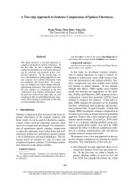
Fig. 4 shows a confusion matrix of the 48 phones
used in TIMIT and the sub-word units learned from
3696 TIMIT utterances. Each circle represents a
mapping pair for a cluster label and an English
phone. The confusion matrix demonstrates a strong

6
In the future, we plan to extend the model and infer the
values of these hyperparameters from data directly.
0
5
10
15
20
25
30
35
40
45
50
55
60
65
70
75
80
85
90
95
100
105
110
115
120
iy
ix

ih
ey
eh
y
ae
ay
aw
aa
ao
ah
ax
uh
uw
ow
oy
w
l
el
er
r
m
n
en
ng
z
s
zh
sh
ch
jh

hh
v
f
dh
th
d
b
dx
g
vcl
t
p
k
cl
epi
sil


Figure 4: A confusion matrix of the learned cluster labels
from the TIMIT training set excluding the sa type utter-
ances and the 48 phones used in TIMIT. Note that for
clarity, we show only pairs that occurred more than 200
times in the alignment results. The average co-occurrence
frequency of the mapping pairs in this figure is 431.
correlation between the cluster labels and individ-
ual English phones. For example, clusters 19, 20
and 21 are mapped exclusively to the vowel /ae/. A
more careful examination on the alignment results
shows that the three clusters are mapped to the same
vowel in a different acoustic context. For example,

cluster 19 is mapped to /ae/ followed by stop conso-
nants, while cluster 20 corresponds to /ae/ followed
by nasal consonants. This context-dependent rela-
tionship is also observed in other English phones
and their corresponding sets of clusters. Fig. 4 also
shows that a cluster may be mapped to multiple En-
glish phones. For instance, clusters 85 and 89 are
mapped to more than one phone; nevertheless, a
closer look reveals that these clusters are mapped to
/n/, /d/ and /b/, which are sounds with a similar place
of articulation (i.e. labial and dental). These corre-
lations indicate that our model is able to discover the
phonetic composition of a set of speech data without
any language-specific knowledge.
The performance of the four acoustic models on
the spoken term detection task is presented in Ta-
ble 2. The English triphone model achieves the best
P@N and EER results and performs slightly bet-
ter than the English monophone model, which indi-
cates a correlation between the quality of an acous-
tic model and its performance on the spoken term
detection task. Although our unsupervised model
does not perform as well as the supervised English
47
unit(%) P@N EER
English triphone 75.9 11.7
English monophone 74.0 11.8
Thai monophone 56.6 14.9
Our model 63.0 16.9
Table 2: The performance of our model and three super-

vised acoustic models on the spoken term detection task.
acoustic models, it generates a comparable EER and
a more accurate detection performance for top hits
than the Thai monophone model. This indicates that
even without supervision, our model captures and
learns the acoustic characteristics of a language au-
tomatically and is able to produce an acoustic model
that outperforms a language-mismatched acoustic
model trained with high supervision.
Table 3 shows that our model improves P@N by
a large margin and generates only a slightly worse
EER than the GMM baseline on the spoken term
detection task. At the end of the training process,
our model induced 169 HMMs, which were used to
compute posteriorgrams. This seems unfair at first
glance because Zhang and Glass (2009) only used
50 Gaussians for decoding, and the better result of
our model could be a natural outcome of the higher
complexity of our model. However, Zhang and
Glass (2009) pointed out that using more Gaussian
mixtures for their model did not improve their model
performance. This indicates that the key reason for
the improvement is our joint modeling method in-
stead of simply the higher complexity of our model.
Compared to the DBM baseline, our model pro-
duces a higher EER; however, it improves the rel-
ative detection precision of top hits by 24.3%. As
indicated in (Zhang et al., 2012), the hierarchical
structure of DBM allows the model to provide a
descent posterior representation of phonetic units.

Even though our model only contains simple HMMs
and Gaussians, it still achieves a comparable, if not
better, performance as the DBM baseline. This
demonstrates that even with just a simple model
structure, the proposed learning algorithm is able
to acquire rich phonetic knowledge from data and
generate a fine posterior representation for phonetic
units.
Table 4 summarizes the segmentation perfor-
mance of the baselines, our model and the heuristic
unit(%) P@N EER
GMM (Zhang and Glass, 2009) 52.5 16.4
DBM (Zhang et al., 2012) 51.1 14.7
Our model 63.0 16.9
Table 3: The performance of our model and the GMM
and DBM baselines on the spoken term detection task.
unit(%) Recall Precision F-score
Dusan (2006) 75.2 66.8 70.8
Qiao et al. (2008)* 77.5 76.3 76.9
Our model 76.2 76.4 76.3
Pre-seg 87.0 50.6 64.0
Table 4: The segmentation performance of the baselines,
our model and the heuristic pre-segmentation on TIMIT
training set. *The number of phone boundaries in each
utterance was assumed to be known in this model.
pre-segmentation (pre-seg) method. The language-
independent pre-seg method is suitable for seeding
our model. It eliminates most unlikely boundaries
while retaining about 87% true boundaries. Even
though this indicates that at best our model only

recalls 87% of the true boundaries, the pre-seg re-
duces the search space significantly. In addition,
it also allows the model to capture proper phone
durations, which compensates the fact that we do
not include any explicit duration modeling mecha-
nisms in our approach. In the best semi-supervised
baseline model (Qiao et al., 2008), the number of
phone boundaries in an utterance was assumed to
be known. Although our model does not incorpo-
rate this information, it still achieves a very close
F-score. When compared to the baseline in which
the number of phone boundaries in each utterance
was also unknown (Dusan and Rabiner, 2006), our
model outperforms in both recall and precision, im-
proving the relative F-score by 18.8%. The key dif-
ference between the two baselines and our method
is that our model does not treat segmentation as a
stand-alone problem; instead, it jointly learns seg-
mentation, clustering and acoustic units from data.
The improvement on the segmentation task shown
by our model further supports the strength of the
joint learning scheme proposed in this paper.
8 Conclusion
We present a Bayesian unsupervised approach to the
problem of acoustic modeling. Without any prior
48
knowledge, this method is able to discover phonetic
units that are closely related to English phones, im-
prove upon state-of-the-art unsupervised segmenta-
tion method and generate more precise spoken term

detection performance on the TIMIT dataset. In the
future, we plan to explore phonological context and
use more flexible topological structures to model
acoustic units within our framework.
Acknowledgements
The authors would like to thank Hung-an Chang and
Ekapol Chuangsuwanich for training the English
and Thai acoustic models. Thanks to Matthew John-
son, Ramesh Sridharan, Finale Doshi, S.R.K. Brana-
van, the MIT Spoken Language Systems group and
the anonymous reviewers for helpful comments.
References
Chun-An Chan and Lin-Shan Lee. 2011. Unsupervised
hidden Markov modeling of spoken queries for spo-
ken term detection without speech recognition. In Pro-
ceedings of INTERSPEECH, pages 2141 – 2144.
Steven B. Davis and Paul Mermelstein. 1980. Com-
parison of parametric representations for monosyllabic
word recognition in continuously spoken sentences.
IEEE Trans. on Acoustics, Speech, and Signal Pro-
cessing, 28(4):357–366.
Sorin Dusan and Lawrence Rabiner. 2006. On the re-
lation between maximum spectral transition positions
and phone boundaries. In Proceedings of INTER-
SPEECH, pages 1317 – 1320.
Yago Pereiro Estevan, Vincent Wan, and Odette Scharen-
borg. 2007. Finding maximum margin segments in
speech. In Proceedings of ICASSP, pages 937 – 940.
Emily Fox, Erik B. Sudderth, Michael I. Jordan, and
Alan S. Willsky. 2011. A sticky HDP-HMM with

application to speaker diarization. Annals of Applied
Statistics.
Alvin Garcia and Herbert Gish. 2006. Keyword spotting
of arbitrary words using minimal speech resources. In
Proceedings of ICASSP, pages 949–952.
John S. Garofolo, Lori F. Lamel, William M. Fisher,
Jonathan G. Fiscus, David S. Pallet, Nancy L.
Dahlgren, and Victor Zue. 1993. Timit acoustic-
phonetic continuous speech corpus.
Andrew Gelman, John B. Carlin, Hal S. Stern, and Don-
ald B. Rubin. 2004. Bayesian Data Analysis. Texts
in Statistical Science. Chapman & Hall/CRC, second
edition.
James Glass. 2003. A probabilistic framework for
segment-based speech recognition. Computer Speech
and Language, 17:137 – 152.
Sharon Goldwater. 2009. A Bayesian framework for
word segmentation: exploring the effects of context.
Cognition, 112:21–54.
Aren Jansen and Kenneth Church. 2011. Towards un-
supervised training of speaker independent acoustic
models. In Proceedings of INTERSPEECH, pages
1693 – 1696.
Frederick Jelinek. 1976. Continuous speech recogni-
tion by statistical methods. Proceedings of the IEEE,
64:532 – 556.
Sawit Kasuriya, Virach Sornlertlamvanich, Patcharika
Cotsomrong, Supphanat Kanokphara, and Nattanun
Thatphithakkul. 2003. Thai speech corpus for Thai
speech recognition. In Proceedings of Oriental CO-

COSDA, pages 54–61.
Kai-Fu Lee and Hsiao-Wuen Hon. 1989. Speaker-
independent phone recognition using hidden Markov
models. IEEE Trans. on Acoustics, Speech, and Sig-
nal Processing, 37:1641 – 1648.
Chin-Hui Lee, Frank Soong, and Biing-Hwang Juang.
1988. A segment model based approach to speech
recognition. In Proceedings of ICASSP, pages 501–
504.
Kevin P. Murphy. 2007. Conjugate Bayesian analysis of
the Gaussian distribution. Technical report, University
of British Columbia.
Radford M. Neal. 2000. Markov chain sampling meth-
ods for Dirichlet process mixture models. Journal
of Computational and Graphical Statistics, 9(2):249–
265.
Yu Qiao, Naoya Shimomura, and Nobuaki Minematsu.
2008. Unsupervised optimal phoeme segmentation:
Objectives, algorithms and comparisons. In Proceed-
ings of ICASSP, pages 3989 – 3992.
Carl Edward Rasmussen. 2000. The infinite Gaussian
mixture model. In Advances in Neural Information
Processing Systems, 12:554–560.
Odette Scharenborg, Vincent Wan, and Mirjam Ernestus.
2010. Unsupervised speech segmentation: An analy-
sis of the hypothesized phone boundaries. Journal of
the Acoustical Society of America, 127:1084–1095.
Balakrishnan Varadarajan, Sanjeev Khudanpur, and Em-
manuel Dupoux. 2008. Unsupervised learning of
acoustic sub-word units. In Proceedings of ACL-08:

HLT, Short Papers, pages 165–168.
Yaodong Zhang and James Glass. 2009. Unsuper-
vised spoken keyword spotting via segmental DTW
on Gaussian posteriorgrams. In Proceedings of ASRU,
pages 398 – 403.
Yaodong Zhang, Ruslan Salakhutdinov, Hung-An Chang,
and James Glass. 2012. Resource configurable spoken
query detection using deep Boltzmann machines. In
Proceedings of ICASSP, pages 5161–5164.
49