Comparison of classification algorithm
Bạn đang xem bản rút gọn của tài liệu. Xem và tải ngay bản đầy đủ của tài liệu tại đây (615.63 KB, 11 trang )
Comparison of Classification
algorithms
datumguy.com
10 mins read
T
here are various different classification algorithms out there
in machine learning which we can use to solve classification
problems. There are some inherent advantages and
disadvantages of using one over another. It also depends on the type
of data we are dealing with. Say, If the data is linearly separable then
logistic regression and support vector machines seem to do the
almost similar job. Now, if the data is non-linearly separable, then
kernel SVM might do the job. On the other hand, if we have a data
which is having some inherent dependence of future events on past
events (for example in text data, the next word is dependent upon the
last word), in such cases naive Bayes does a good job. Like in the
problem of spam detection or anything related to text, naive Bayes is
a go-to algorithm for these tasks.
1. Naive Bayes Algorithms
Naive Bayes Algorithm is one of the most simplest algorithms for
solving classification machine learning problems. It uses a very
important concepts in statistics and probability known as Bayes’
Theorem. With new information, usually the measure of probability
improves. This basic fact is an underlying concept in Bayes' Theorem
which is a subject matter of statistics. Assume a situation in which
there is some prior probability of the happening of an event and with
new information, we can compute what is called as posterior
probability. The posterior probability usually is a better and improved
probability over the prior probability. The probability of raining on an
usual day is ½ (which puts us in confusion) but what is the
probability of raining given that the day is sunny or what is the
probability of raining given that the day is cloudy. Intuitively, In the
first case, the probability will be lower whereas it will be higher in
the latter (In both of these cases the posterior probability is improved
estimate of probability than the prior). This is exactly what is
accomplished by Bayes Theorem. The data is available and that data
can be transformed into a contingency table through which various
probabilities can be computed.
Some points
• The Naive Bayes algorithm is considered naive because it
assumes the independence between independent variables.
The reason this assumption is important is that we need to
compute the joint likelihood of the variables which can be
just obtained by multiplying the respective probabilities if
the variables are assumed, independent. But in real life, this
assumption rarely holds true. Even in those cases, the naive
Bayes algorithms can be used without affecting the results
that much.
• One of the reasons that this algorithm is so popular and is
used widely in the research as well as in the industry is
because of its simplicity and ease of implementation.
• One of the main disadvantages of the Naive Bayes algorithm
is that they make some assumptions that are too simple in
general and they are hardly true in real life. In real life, the
features are hardly independent.
2. Logistic Regression
The logistic regression is one another method for obtaining a
prediction for the response variable of the discrete class. The term
regression should not confuse it with normal regression. The subject
of linear and logistic regression have been quite heavily used in
statistics as well. The term logistic regression is used because of
historical reasons. One reason that can explain this name is the
simultaneous development of linear and logistic regression in
statistics. Here regression might just tell that we are dealing with a
problem involving prediction or using data to predict things. The
term linear means the link function used in linear regression is linear
while in the logistic, it's a function known as Logistic. The further
theoretical aspects of this article are beyond the scope of this article
but you are encouraged to look for it online. Statistics often looks at
these two problems in a little bit similar contexts. In statistics, both
are said to come under the section of prediction of a response based
on data. The difference arises in the type of response that we want to
predict. Say, I have to predict a continuous output, then linear
regression is used while on the other hand when the class of response
is discrete, then we use logistic regression in those situations (why
can't we just use linear in these cases?). There is this notion of
response random variable in statistics. In linear regression, this
response variable follows a normal distribution while in the logistic
model it follows a Bernoulli distribution. The Bernoulli distribution is
a distribution used to model the success or failures of a real situation.
Say, if we take a problem of classifying the mail as spam or not. In
this case, the variable can be regarded as coming from a Bernoulli
distribution where the success might correspond to a mail being spam
while failure can be considered an example to be non-spam.
Consequently, the function that we estimate parameters of, changes.
In the linear regression, this function is linear in parameters while in
the logistic regression this has to change as if we use the same
function for this problem, the expected output that we get might be
very large (larger than 1) or very small (smaller than 0). But what we
expect is to get something between 0 and 1, it is because the expected
value of Bernoulli distribution is p which stands for the probability of
success and probability always lies between 0 and 1. The shape of the
logistic function for which we learn parameters is as follows (Note
that this function is linear in case of linear regression):
Some points
• Logistic Regression outputs a probability of a class given
some inputs.
• It is only used for binary response variables as we assume
that the response will follow Bernoulli distribution.
• In machine learning, the way we take care of more than two
categories is something that is known as One Vs Rest
Classifier Approach. In this approach, a binary model is
trained k time where k is no of unique class. In each of the
training, we consider one class as 1 and the rest of the class
as 0 which we do for K times. While making a prediction,
we pass our input through all of these models (k in this
case) and choose the one which is occurring the maximum
number of times.
3. K Nearest Neighbour
Consider a situation where you are struggling with the decision to
purchase which car out of the two available options to purchase.
Suppose you decided to ask your neighbors for this decision. There
are many neighbors who live nearby. You restrict yourself with only
10 neighbors. When you take their suggestion, then out of the 10, 8
suggest you purchase car number 1 and 2 suggest you purchase car
number 2. Which car are you more likely to purchase if you were to
base your decision purely on the basis of your neighbor's response.
Then, the answer is undoubtedly the car number 1.
This exact intuition is used in one of the algorithms of classification
known as K-nearest neighbors. Consider the following scatter where
blue squares represent one class while the red triangle represents
another class. The question mark is the input that we want to get the
class of:
We have decided to base our decision on three most near point and
you can clearly see that out the tree points two are triangles and one
is square. Hence, the unknown class is the red one.
In the prediction of the new examples, K nearest neighbor algorithms
use the voting method. The parameter K represents the number of
neighbors to base our decision on, which we can tweak. Say, we want
to take K as 6, that means when classifying new data point, we will
look at the nearby 6 points and the class which is more frequent in
those 6 will be predicted. Now, there is one more problem, the
problem of finding the top k nearest points. This can be easily solved
using the so-called Euclidean distance metric. We can compute the
distance of the new data point from each of our training data points
and choose the top 6 which are having low distance with the new
point. This poses a new problem for us. In the K-nearest neighbors, at
each prediction we need to have the training data set unlike other
algorithms where once trained, we can just use the new data point in
the model and get the output (we don't necessarily have to keep the
whole of training data in each prediction because we are learning a
function after which we can get rid of data if we want). This is why
the K nearest neighbors algorithm is often known as the lazy learning
algorithm because it does not try to generalize the training data to a
functional form rather it will always start doing the same steps again
and again when it has to make prediction and those steps will be once
again repeated once new data point arrives which often makes it an
attractive algorithm when the data is constantly getting updated.
Some Points
• K is the only parameter that is required to be tweaked in
this algorithm.
• It is one of the most interpretable algorithms in machine
learning. In terms of interpretability, one other such
algorithm is the decision tree.
• The whole data is required at the time of making a new
prediction. The reason for this is that K nearest algorithm
comes under the collection of non-parametric algorithms for
which the algorithm does not learn any specific function.
• The machine learning techniques like linear and logistic
where they learn some function comes under the class of
parametric algorithm.
4. Decision Tree
If someone asks me, tell me one algorithm which is most intuitive in
the large collection of machine learning algorithms, then my answer
would undoubtedly be decision trees. This is because of the fact that
this algorithm makes a prediction just the way how we human make a
prediction in our day to day world. Consider an example in which we
need to decide whether we need to take an umbrella with us not.
First, we will ask how is the weather like? If it's cloudy, then the
probability of taking an umbrella with us should increase. This is how
decision trees work by asking some questions related to features of
the data to segregate the data into a smaller and smaller part. Now,
one natural question arises how does the decision tree decides which
variable to segregate our data on and what will be the point at which
we segregate that variable. The answer is the maximization of
entropy (measure and f impurity of a particular split). The math is
beyond the scope of this article but you are encouraged to look for it
online. There are two broad questions that at each split need to be
answered:
• Which feature should be used to make the split?
• what value should the data be split on?
These two questions can be answered using something called an
impurity measure at each split. At each split, this measure needs to be
evaluated and need to be compared with all the set of impurities. We
choose that feature and value combination which has the lowest
impurity. Obviously, it is a computationally challenging task but the
modern computer can handle this quite effectively.
Some points
• It is most interpretable algorithms available out there. You
can literally track down how a decision tree makes the
prediction.
• If we continue to train the data using decision trees, then it
will overfit the training data because at the end (In the leaf
nodes), there will only be one example per node and the
tree will just learn the training data well but it will fail to
generalize beyond the scope of train data set.
• In the above-mentioned situation, we can go for pruning the
tree. Pruning means to kind of cut down the tree at some
predefined point. This means we decide beforehand how
long will our tree be.
• The decision tree can be used in solving two different class
of problems. It can be used to solve regression problems
also apart from classification problems.
• The decision tree can be used to select the best features for
our model even in other algorithms
• We don't have to think about scaling the features, even if
some features are simply irrelevant, then also the decision
tree will find the best subset of features for training.
• The way decision tree makes a prediction is it will ask a
bunch of questions about the data based on a particular
feature and it will continue to split the data by asking these
types of questions until we are sure about which class a
particular node belongs to. The following is a nice
representation of the decision tree:
5. Random forest
If you understand the decision tree, then you will have not much
difficulty understanding the random forest. You can think of the
random forest as the collection of decision trees which is also true in
general sense. There can be two different forms of random forest just
like there are two different types of decision trees, one for
classification and one for regression. We will restrict our attention to
classification only.
Some Points
• Random forest is nothing but the collection of many
decision trees.
• Just like decision trees, the random forest can also be of two
forms. One for regression and one for classification.
• It is often called an ensemble learning method because it
combines many decision trees.
• It outperforms the decision tree and less prone to overfit the
data. It is less prone to overfit is it reduces the variance of
the decision trees.
• We don't have to think about scaling the features, even if
some features are simply irrelevant, then also the random
forest works just fine.
• Random forest is less interpretable than decision trees but
can produce really powerful results.
• The random forest can look something like the following
where we have chosen three trees:
6. Support Vector Machines
Support Vector Machine is one another classification machine
learning algorithm which is quite popular both in academia and
industry. The popularity of the algorithm comes from the fact that it
has been proven to outperform other sophisticated algorithms for
certain tasks. In the task of digits recognition, for example, it has
been seen that the performance is at par with algorithms like neural
networks which takes a lot of time to train. It is a very intuitive
algorithm which works by maximizing the so-called margin of the
two classes. This can be best represented by the following
classification diagram:
It works for only linearly separable data but there are some
techniques by which it can accommodate even nonlinear cases.
Some Points
• When training data is less, the algorithm works like a
charm, there is no need to use algorithms like neural
networks which will have interpretability problems.
• When the data is linearly separable, one can use this
algorithm but it is not advisable as the real power of
support vector machines is seen in the nonlinear cases. In
linear cases, there are other algorithms which work just
fine. In fact, in the linearly separable data case, the logistic
regression and support vector machines almost work the
same.
• It's used widely in image recognition tasks because of its
low cost of training.
We have come to the end of this blog. I hope, I was able to explain
the key components that differentiate various classification
algorithms. You are encouraged to explore any topic that excites
you more. I have explained the key components that make up the
algorithms and some of the points that are worth noting.
Thank You.