A Crash Course on Reinforcement Learning

A Crash Course on Reinforcement Learning
Farnaz Adib Yaghmaie

∗

arXiv:2103.04910v1 [cs.LG] 8 Mar 2021

Department of Electrical Engineering, Linköping University,
Linköping, Sweden.
Lennart Ljung†
Department of Electrical Engineering, Linköping University,
Linköping, Sweden.
March 9, 2021

Abstract
The emerging field of Reinforcement Learning (RL) has led to impressive results in varied
domains like strategy games, robotics, etc. This handout aims to give a simple introduction to
RL from control perspective and discuss three possible approaches to solve an RL problem: Policy
Gradient, Policy Iteration, and Model-building. Dynamical systems might have discrete actionspace like cartpole where two possible actions are +1 and -1 or continuous action space like linear
Gaussian systems. Our discussion covers both cases.

1

Introduction

Machine Learning (ML) has surpassed human performance in many challenging tasks like pattern
recognition [1] and playing video games [2]. By recent progress in ML, specifically using deep networks,
there is a renewed interest in applying ML techniques to control dynamical systems interacting with
a physical environment [3, 4] to do more demanding tasks like autonomous driving, agile robotics [5],
solving decision-making problems [6], etc.
Reinforcement Learning (RL) is one of the main branches of Machine Learning which has led to

impressive results in varied domains like strategy games, robotics, etc. RL concerned with intelligent
decision making in a complex environment in order to maximize some notion of reward. Because of
its generality, RL is studied in many disciplines such as control theory [7–10] and multi-agent systems
[11–15, 15–20], etc. RL algorithm have shown impressive performances in many challenging problems
including playing Atari games [2], robotics [5,21–23], control of continuous-time systems [3,7,8,24–31],
and distributed control of multi-agent systems [11–13, 17].
From control theory perspective, a closely related topic to RL is adaptive control theory which
studies data-driven approaches for control of unknown dynamical systems [32,33]. If we consider some
notion of optimality along with adaptivity, we end up in the RL setting where it is desired to control
an unknown system adaptively and optimally. The history of RL dates back decades [34, 35] but by
recent progress in ML, specifically using deep networks, the RL field is also reinvented.
In a typical RL setting, the model of the system is unknown and the aim is to learn how to
react with the system to optimize the performance. There are three possible approaches to solve
∗ email:
† email:




1


an RL problem [9]. 1- Dynamic Programming (DP)-based solutions: This approach relies on
the principle of optimal control and the celebrated Q-learning [36] algorithm is an example of this
category. 2- Policy Gradient: The most ambitious method of solving an RL problem is to directly
optimize the performance index [37]. 3- Model-building RL: The idea is to estimate a model
(possibly recursively) [38] and then the optimal control problem is solved for the estimated model.
This concept is known as adaptive control [33] in the control community, and there is vast literature
around it.
In RL setting, it is important to distinguish between systems with discrete and continuous action

spaces. A system with discrete action space has a finite number of actions in each state. An example is
the cartpole environment where a pole is attached by an un-actuated joint to a cart [39]. The system
is controlled by applying a force of +1 or -1 to the cart. A system with continuous action space has
an infinite number of possible actions in each state. Linear quadratic (LQ) control is a well studied
example where continuous actions space can be considered [24,25]. The finiteness or infiniteness of the
number of possible actions makes the RL formulation different for these two categories and as such it
is not straightforward to use an approach for one to another directly.
In this document, we give a simple introduction to RL from control perspective and discuss three
popular approaches to solve RL problems: Policy Gradient, Q-learning (as an example of Dynamic
Programming-based approach) and model-building method. Our discussion covers both systems with
discrete and continuous action spaces while usually the formulation is done for one of these cases.
Complementary to this document is a repository called A Crash Course on RL, where one can run the
policy gradient and Q-learning algorithms on the cartpole and linear quadratic problems.

1.1

How to use this handout?

This handout aims to acts as a simple document to explain possible approaches for RL. We do not
give expressions and equations in their most exact and elegant mathematical forms. Instead, we try
to focus on the main concepts so the equations and expressions may seem sloppy. If you are interested
in contributing to the RL field, please consider this handout as a start and deploy exact notation in
excellent RL references like [34, 40].
An important part of understanding RL is the ability to translate concepts to code. In this document, we provide some sample codes (given in shaded areas) to illustrate how a concept/function is
coded. Except for one example in the model-building approach on page 23 which is given in MATLAB syntax (since it uses System Identification toolbox in MATLAB), the coding language in this
report is Python. The reason is that Python is currently the most popular programming language
in RL. We use TensorFlow 2 (TF2) and Keras for the Machine Learning platforms. TensorFlow 2 is
an end-to-end, open-source machine learning platform and Keras is the high-level API of TensorFlow
2: an approchable, highly-productive interface for solving machine learning problems, with a focus
on modern deep learning. Keras empowers engineers and researchers to take full advantage of the

scalability and cross-platform capabilities of TensorFlow 2. The best reference for understanding the
deep learning elements in this handout is Keras API reference. We use OpenAI Gym library which is
a toolkit for developing and comparing reinforcement learning algorithms [41] in Python.
The python codes provided in this document are actually parts of a repository called A Crash
Course on RL
/>You can run the codes either in your web browser or in a Python IDE like PyCharm.
How to run the codes in web browser? Jupyter notebook is a free and interactive web tool known
as a computational notebook, which researchers can use to combine python code and text. One can
run Jupyter notebooks (ended with *.ipynb) on Google Colab using web browser. You can run the
code by following the steps below:
1. Go to
2


/>and sign in with a Google account.
2. Click “File", and select “Upload Notebook". If you get the webpage in Swedish, click “Arkiv"
and then “Ladda upp anteckningsbok".
3. Then, a window will pop up. Select Github, paste the following link and click search
/>4. Then, a list of files with type .ipynb appears. They are Jupyter notebooks. Jupyter notebooks
can have both text and code and it is possible to run the code. As an example, scroll down and
open “pg_on_cartpole_notebook.ipynb".
5. The file contains some cells with text and come cells with code. The cells which contain code
have [ ] on the left. If you move your mouse over [ ], a play box appears. You can click on it
to run the cell. Make sure not to miss a cell as it causes fatal errors.
6. You can continue like this and run all code cells one by one up to the end.
How to run the codes in PyCharm? You can follow these steps to run the code in a Python IDE
(preferably PyCharm)
1. Go to
/>and clone the project.
2. Open PyCharm. From PyCharm. Click File and open project. Then, navigate to the project

folder.
3. Follow Preparation.ipynb notebook in “A Crash Course on RL” repository to build a virtual
environment and import required libraries.
4. Run the python file (ended with .py) you want.

1.2

Important notes to the reader

It is important to keep in mind that, the code provided in this document is for illustration purpose;
for example, how a concept/function is coded. So do not get lost in Python-related details. Try to
focus on how a function is written: what are the inputs? what are the outputs? how this concept is
coded? and so on.
The complete code can be found in A Crash Course on RL repository. The repository contains
coding for two classical control problems. The first problem is the cartpole environment which is an
example of systems with discrete action space [39]. The second problem is Linear Quadratic problem
which is an example of systems with continuous action space [24, 25]. Take the Linear Quadratic
problem as a simple example where you can do the mathematical derivations by some simple (but
careful) hand-writing. Summaries and simple implementation of the discussed RL algorithms for the
cartpole and LQ problem are given in Appendices A-B. The appendices are optional, you can skip
reading them and study the code directly.
We have summarized the frequently used notations in Table 1.

3


Table 1: Notation
General:
[.]†

Transpose operator

< S, A, P, R, γ >

A Markov Decision Process with state set S,
action set A, transition probability set P, immediate reward set R and discount factor γ

ns

Number of states for discrete state space or
dimension of states in continuous action space

na

Number of actions for discrete action space or
the dimension of action in continuous action
space

θ

The parameter vector to be learned

π(θ)

Deterministic policy or probability density
function of the policy (with parameter vector
θ)

The subscript t

The time step

st , at

The state and action at time t

rt = r(st , at )

The immediate reward

ct = −rt

The immediate cost

R(T )

Total reward in form of discounted (3), undiscounted (6) or averaged (4).

τ, T

A trajectory and the trajectory length

P (τ |θ)

Probability of trajectory τ conditioned on θ

p(at |θ)

evaluation of the parametric pdf πθ at at (likelihood)

V, Q

The value function and the Q-function

G
vecs(G) = [g11 , ..., g1n , g22 ,

The kernel of quadratic Q = z † Gz

Policy
Gradient:

Qlearning:

The vectorization of the upper-triangular part
of a symmetric matrix G ∈ Rn×n

..., g2n , ..., gnn ]†
vecv(v) = [v12 , 2v1 v2 , ..., 2v1 vn ,

The quadratic vector of the vector v ∈ Rn

v22 , ..., 2v2 vn , ..., vn2 ]†

4


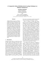
Figure 1: An RL framework. Photo Credit: @ />
2

What is Reinforcement Learning

Machine learning can be divided into three categories: 1- Supervised learning, 2- Unsupervised learning,
and 3- Reinforcement Learning (RL). Reinforcement Learning (RL) is concerned with decision making
problem. The main thing that makes RL different from supervised and unsupervised learning is that
data has a dynamic nature in contrast to static data sets in supervised and unsupervised learning. The
dynamic nature of data means that data is generated by a system and the new data depends on the
previous actions that the system has received. The most famous definition of RL is given by Sutton
and Barto [34] “Finding suitable actions to take in a given situation in order to maximize a reward".
The idea can be best described by Fig. 1. We start a loop from the agent. The agent selects
an action and applies it to the environment. As a result of this action, the environment changes and
reveals a new state, a representation of its internal behavior. The environment reveals a reward which
quantifies how good was the action in the given state. The agent receives the state and the reward and
tries to select a better action to receive a maximum total of rewards in future. This loop continues
forever or the environment reveals a final state, in which the environment will not move anymore.
As we noticed earlier, there are three main components in an RL problem: Environment, reward,
and the agent. In the sequel, we introduce these terms briefly.

2.1

Environment

Environment is our dynamical system that produces data. Examples of environments are robots, linear
and nonlinear dynamical systems (in control theory terminology), and games like Atari and Go. The
environment receives an action as the input and generates a variable; namely state; based on its own
rules. The rules govern the dynamical model and it is assumed to be unknown. An environment is
usually represented by a Markov Decision Process (MDP). In the next section, we will define MDP.

2.2

Reward

Along with each state-action pair, the environment reveals a reward rt . Reward is a scalar measurement
that shows how good was the action at the state. In RL, we aim to maximize some notion of reward;
for example, the total reward where 0 ≤ γ ≤ 1 is the discount or forgetting factor
T

γ t rt .

R=
t=1

5


2.3

Agent

Agent is what we code. It is the decision-making center that produces the action. The agent receives
the state and the reward and produces the action based on some rules. We call such rules policy and
the agent updates the rules to have a better one.
2.3.1

Agent’s components

An RL agent can have up to three main components. Note that the agent need not have all but at
least one.
• Policy: The policy is the agent’s rule to select action in a given state. So, the policy is a map
π : S → A from the set of states S to set of actions A. Though not conceptually correct, it is

common to use the terms “Agent" and “Policy" interchangeably.
• Value function: The value function quantifies the performance of the given policy. It quantifies
the expected total reward if we start in a state and always act according to policy.
• Model: The agent’s interpretation of the environment.
2.3.2

Categorizing RL agent

There are many ways to categorize an RL agent, like model-free and model-based, online or offline
agents, and so on. One possible approach is to categorize RL agents based on the main components
that the RL agent is built upon. Then, we will have the following classification
• Policy gradient.
• Dynamic Programming (DP)-based solutions.
• Model building.
Policy gradient approaches are built upon defining a policy for the agent, DP-based solutions require
estimating value functions and model-building approaches try to estimate a model of the environment.
This is a coarse classification of approaches; indeed by combining different features of the approaches,
we get many useful variations which we do not discuss in this handout.
All aforementioned approaches reduce to some sort of function approximation from data obtained
from the dynamical systems. In policy gradient, we fit a function to the policy; i.e. we consider policy
as a function of state π = network(state). In DP-based approach, we fit a model to the value function
to characterize the cost-to-go. In the model-building approach, we fit a model to the state transition
of the environment.
As you can see, in all approaches, there is a modeling assumption. The thing which makes one
approach different from another is “where” to put the modeling assumption: policy, value function or
dynamical system. The reader should not be confused by the term “model-free” and think that no
model is built in RL. The term “model-free” in RL community is simply used to describe the situation
where no model of the dynamical system is built.

3

Markov Decision Process

A Markov decision process (MDP) provides a mathematical framework for modeling decision making
problems. MDPs are commonly used to describe dynamical systems and represent environment in the
RL framework. An MDP is a tuple < S, A, P, R, γ >
• S: The set of states.
• A: The set of actions.
6


• P: The set of transition probability.
• R: The set of immediate rewards associated with the state-action pairs.
• 0 ≤ γ ≤ 1: Discount factor.

3.1

States

It is difficult to define the concept of state but we can say that a state describes the internal status of
the MDP. Let S represent the set of states. If the MDP has a finite number of states, |S| = ns denotes
the number of states. Otherwise, if the MDP has a continuous action space, ns denote the dimension
of the state vector.
In RL, it is common to define a Boolean variable done for each state s visited in the MDP

done(s) =

T rue, s is the final state or the MDP needs to be restarted after s
F alse, Otherwise.

This variable is True only if the state is a final state in the MDP: if the MDP goes to this state, the
MDP stays there forever or the MDP needs to be restarted. The variable done is False otherwise.
Defining done comes handy in developing RL algorithms.

3.2

Actions

Actions are possible choices in each state. If there is no choice at all to make, then we have a Markov
Process. Let A represent the set of actions. If the MDP has a finite number of actions, |A| = na
denotes the number of actions. Otherwise, if the MDP has a continuous action space, na denotes the
dimension of the actions. In RL, it is crucial to distinguish between MDPs with discrete or continuous
action spaces as the methodology to solve will be different.

3.3

Transition probability

The transition probability describes the dynamics of the MDP. It shows the transition probability from
all states s to all successor states s for each action a. P is the set of transition probability with na
matrices each of dimension ns × ns where the s, s entry reads
[P a ]ss = p[st+1 = s |st = s, at = a].

(1)

One can verify that the row sum is equal to one.

3.4

Reward

The immediate reward or reward in short is measure of goodness of action at at state st and it is
represented by
rt = E[r(st , at )]

(2)

where t is the time index and the expectation is calculated over the possible rewards. R represent
the set of immediate rewards associated with all state-action pairs. In the sequel, we give an example
where r(st , at ) is stochastic but throughout this handout, we assume that the immediate reward is
deterministic and no expectation is involved in (2).
The total reward is defined as
T

γ t rt ,

R(T ) =
t=1

where γ is the discount factor which will be introduced shortly.
7

(3)


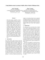
Figure 2: A Markov Decision Process. The photo is a modified version of the photo in @
wiki/Markov_decision_process

3.5

Discount factor

The discount factor 0 ≤ γ ≤ 1 quantifies how much we care about the immediate rewards and future
rewards. We have two extreme cases where γ → 0 and γ → 1.
• γ → 0: We only care about the current reward not what we’ll receive in future.
• γ → 1: We care all rewards equally.
The discounting factor might be given or we might select it ourselves in the RL problem. Usually,
we consider 0 < γ < 1 and more closely to one. We can select γ = 1 in two cases. 1) There exists an
absorbing state in the MDP such that if the MDP is in the absorbing state, it will never move from it.
2) We care about the average cost; i.e. the average of energy consumed in a robotic system. In that
case, we can define the average cost as
1
T →∞ T

T

(4)

rt .

R(T ) = lim

t=1

Example 3.1 Consider the MDP in Fig. 2. This MDP has three states S = {s0 , s1 , s2 } and two
actions A = {a0 , a1 }. The rewards for some of the transitions are shown by orange arrows. For
example, if we start at state s1 and take action a0 , we will end up at one of the following cases
• With probability 0.1, the reward is −1 and the next state is s1 .
• With probability 0.7, the reward is +5 and the next state is s0 .
• With probability 0.2, the reward is +5 and the next state is s2

As a result, the reward for state s1 and action a0 reads
E[r(s1 , a0 )] = 0.1 × (−1) + 0.7 × (5) + +0.2 × (5) = 4.4.
The transition probability matrices are

0.5 0


P a0 = 0.7 0.1

0.4 0

given by


0.5
0




a
0.2 , P 1 =  0


0.6
0.3

Observe that the sum of each row in P a0 , P a1 equals to one.
8

0
0.95
0.3

1





0.05 .

0.4


3.6

Revisiting the agents component again

Now that we have defined MDP, we can revisit the agents components and define them better. As we
mentioned an RL agent can have up to three main components.
• Policy: The policy is the agent’s rule to select action in a given state. So, the policy is a map
π : S → A. We can have Deterministic policy a = π(s) or stochastic policy defined by a pdf
π(a|s) = P [at = a|st = s].
• Value function: The value function quantifies the performance of the given policy in the states
V (s) = E rt + γrt+1 + γ 2 rt+2 + ...|st = s .
• Model: The agent’s interpretation of the environment [P a ]ss which might be different from the
true value.
We categorize possible approaches to solve an RL problem based on the main component on which
the agent is built upon. We start with the policy gradient approach in the next section which relies

on building/estimating policy.

4

Policy Gradient

The most ambitious method of solving an RL problem is to directly learn the policy from optimizing
the total reward. We do not build a model of environment and we do not appeal to the Bellman
equation. Indeed our modeling assumption is in considering a parametric probability density function
for the policy and we aim to learn the parameter to maximize the expected total reward
J = Eτ ∼πθ [R(T )]

(5)

where
• πθ is the probability density function (pdf) of the policy and θ is the parameter vector.
• τ is a trajectory obtained from sampling the policy and it is given by
τ = (s1 , a1 , r1 , s2 , a2 , r2 , s3 , ..., sT +1 )
where st , at , rt are the state, action, reward at time t and T is the trajectory length. τ ∼ πθ
means that trajectory τ is generated by sampling actions from the pdf πθ .
• R(T ) is undiscounted finite-time total reward
T

R(T ) =

rt .

(6)

t=1

• Expectation is defined over the probability of the trajectory
We would like to directly optimize the policy by a gradient approach. So, we aim to obtain the gradient
of J with respect to parameter θ
∇θ J.

9


The algorithms that optimizes the policy in this way are called Policy Gradient (PG) algorithms.
The log-derivative trick helps us to obtain the policy gradient ∇θ J. The trick depends on the simple
1
math rule ∇p log p = . Assume that p is a function of θ. Then, using chain rule, we have
p
∇θ log p = ∇p log p∇θ p =

1
∇θ p.
p

Rearranging the above equation
∇θ p = p∇θ log p.

(7)

Equation (7) is called the log-derivative trick and helps us to get rid of dynamics in PG. You will see
an application of (7) in Subsection 4.3.
In the sequel, we define the main components in PG.

4.1

Defining probability density function for the policy

In PG, we consider the class of stochastic policies. One may ask why do we consider stochastic policies
when we know that the optimal policy for MDP is deterministic [9, 42]? The reason is that in PG,
no value function and no model of the dynamics are built. The only way to evaluate a policy is to
deviate from it and see the total reward. So, the burden of the optimization is shifted onto sampling
the policy: By perturbing the policy and observing the result, we can improve policy parameters. If
we consider a deterministic policy in PG, the agent gets trapped in a local minimum. The reason is
that the agent has “no” way of examining other possible actions and furthermore, there is no value
function to show how “good” the current policy is. Considering a stochastic policy is essential in PG.
As a result, our modeling assumption in PG is in considering a probability density function (pdf)
for the policy. As we can see in Fig. 3 the pdf is defined differently for discrete and continuous random
variables. For discrete random variables, the pdf is given as probability for all possible outcomes while
for continuous random variables it is given as a function. This tiny technical point makes coding
completely different for the discrete and continuous action space cases. So we treat discrete and
continuous action spaces differently in the sequel.

Figure 3:
Pdf for discrete and continuous reandom variables.
Photo Credit:
/>
4.1.1

@

Discrete action space

As we said earlier, our modeling assumption in PG is in considering a parametric pdf for the policy. We
represent the pdf with πθ where θ is the parameter. The pdf πθ maps from the state to the probability

of each action. So, if there are na actions, the policy network has na outputs, each representing the
probability of an action. Note that the outputs should sum to 1.

10


Figure 4: An example of network producing the pdf πθ
An example of network is shown in Fig. 4. The network generates the pdf for three possible actions
by taking state as the input. In this figure, p1 is the probability associated with action a1 , p2 associated
with action a2 and p3 is associated with action a3 . Note that it should hold p1 + p2 + p3 = 1.
Generating pdf and sampling an action in discrete action space case
Let πθ be generated by the function network(state)
network = k e r a s . S e q u e n t i a l ( [
k e r a s . l a y e r s . Dense ( 3 0 , input_dim=n_s , a c t i v a t i o n= ’ r e l u ’ ) ,
k e r a s . l a y e r s . Dense ( 3 0 , a c t i v a t i o n= ’ r e l u ’ ) ,
k e r a s . l a y e r s . Dense ( n_a , a c t i v a t i o n= ’ softmax ’ ) ] )
In the above code, the network is built and the parameters of the network (which are biases and
weights) are initialized. The network takes state of dimension ns as the input and uses it in a fully
connected layer with 30 neurons, with the activation function as relu, followed by another layer with
30 neurons and again with the activation function as relu. Then, we have the last layer which has
na number of outputs and we select the activation function as softmax as we want to have the sum
of probability equal to one.
To draw a sample a ∼ πθ , first we feed the state to the network to produce the pdf πθ and then, we
select an action according to the pdf. This can be done by the following lines of code
softmax_out = network ( s t a t e )
a = np . random . c h o i c e ( n_a , p=softmax_out . numpy ( ) [ 0 ] )

4.1.2

Continuous action space

When the action space is continuous, we select the pdf πθ as a diagonal Gaussian distribution πθ =
N (µθ , Σ), where the mean is parametric and the covariance is selected as Σ = σ 2 Ina , with σ > 0 as a
design parameter

11


πθ =

1
(2πσ 2 )na

exp[−

1
(a − µθ (s))† (a − µθ (s))].
2σ 2

As a result, our modeling assumption is in the mean of the pdf, the part that builds our policy µθ . The
actions are then sampled from the pdf πθ = N (µθ , Σ). For example, a linear policy can be represented
by µθ = θs where θ is the linear gain and the actions are sampled from N (θs, σ 2 Ina ).
Sampling an action in continuous action space
Let µθ be generated by the function network(state). That is µθ (s) = network(state) takes the state
variable as the input and has vector parameter θ. To draw a sample a ∼ N (µθ , σIna ), we do the
following
a = network ( s t a t e ) + sigma ∗ np . random . randn (n_a)

4.2

Defining the probability of trajectory

We defined a parametric pdf for the policy in the previous subsection. The next step is to sample
actions from the pdf and generate a trajectory. τ ∼ πθ means that a trajectory of the environment
is generated by sampling action from πθ . Let s1 denote the initial state of the environment. The
procedure is as follows.
1. We sample the action a1 from the pdf; i.e. a1 ∼ πθ . We derive the environment using a1 . The
environment reveals the reward r1 and transits to a new state s2 .
2. We sample the action a2 from the pdf; i.e. a2 ∼ πθ . We derive the environment using a2 . The
environment reveals the reward r2 and transits to a new state s3 .
3. We repeat step 2 for T times and in the end, we get a trajectory
τ = (s1 , a1 , r1 , s2 , a2 , r2 , s3 , ..., sT +1 ).
The probability of the trajectory τ is defined as follows
T

p(st+1 |st , at )p(at |θ).

P (τ |θ) =

(8)

t=1

in which
• p(st+1 |st , at ) represents the dynamics of the environment; it defines the next state st+1 given the
current state st and the current action at . Note that in RL we do NOT know p(st+1 |st , at ). You
will see later that p(st+1 |st , at ) is not needed in the computation.
• p(at |θ) is the likelihood function and it is obtained by evaluating the pdf πθ at at . In the sequel,
we will see how p(at |θ) is defined in discrete and continuous action spaces.
4.2.1

Discrete action space

If the action space is discrete, network(state) denotes the probability density function πθ . It is a vector
with however many entries as there are actions, and the actions are the indices for the vector. So,
p(at |θ) is obtained by indexing into the output vector network(state).
12


4.2.2

Continuous action space

Let the action space be continuous and assume that the dimension is na , we consider a multi-variate
Gaussian with mean µθ (s) =network(state). Then, p(at |θ) is given by
p(at |θ) =

4.3

1
(2πσ 2 )na

exp[−

1
(at − µθ (st ))† (at − µθ (st ))].
2σ 2

(9)

Computing the gradient ∇θ J

The final step in PG which results in learning the parameter vector is to compute the gradient of J
in (5)-(6) with respect to the parameter vector θ; that is ∇θ J. We already have all components to
compute this term. First, we need to do a little math here
∇θ J = ∇θ E [R(T )]
P (τ |θ)R(T ) replacing the expectation with the integral,

= ∇θ
τ

∇θ P (τ |θ)R(T ) bringing the derivative inside,

=

(10)

τ

P (τ |θ)∇θ log P (τ |θ)R(T ) using log-derivative trick (7),

=
τ

= E[∇θ log P (τ |θ)R(T )] replacing the integral with the expectation.
In (10), P (τ |θ) is the probability of the trajectory defined in (7). ∇θ log P (τ |θ) reads
T

T

∇θ log P (τ |θ) = ∇θ

log p(st+1 |st , at ) + ∇θ
t=1

log p(at |θ)
t=1

T

(11)

∇θ log p(at |θ).

=
t=1

The first summation in (11) contains the dynamics of the system log p(st+1 |st , at ) but since it is
independent of θ, it disappears while taking gradient. p(at |θ) is the likelihood function defined in
subsection 4.2 for continuous (see (9)) and discrete action spaces. By substituting (11) in (10) ∇θ J
reads
T

∇θ J = E[R(T )

∇θ log p(at |θ)].

(12)

t=1

This is the main equation in PG. One can replace the expectation with averaging or simply drop the
expectation operator.
4.3.1

Discrete action space

Computing (12) in the discrete action space case is quite simple because we can use a pre-built cost
function in Machine learning libraries. To see this point note that J (without the gradient)
T

R(T ) log p(at |θ)

J=
t=1

13

(13)


is in the form of the weighted cross entropy cost (wcec) function which is used and optimized in the
classification task
Jwcec =

1
M

M

C
c
wc ì ym
ì log(h (xm , c))

(14)

m=1 c=1

where
ã C: number of classes,
• M : number of training data,
• wc : is the weight of class c,
• xm : input for training example m,
c
• ym
: target label for xm for class c,

• hθ : neural network producing probability with parameters θ.
At the first glance, it might seem difficult to recast the performance index (13) to the weighted
cross entropy cost function in (14). But a closer look will verify that it is indeed possible. We aim to
maximize (13) in PG while in the classification task, the aim is to minimize the weighted cross entropy
cost in (14). This resolves the minus sign in (14). na actions are analogous to C categories and the
trajectory length T in (13) is analogous to the number of data M in (14). R(T ) is the weight of class
c
c; i.e. wc . xm is analogous to the state st . ym
is the target label for training example m for class c,
c
ym
=

1 if c is the correct class for xm ,
0 otherwise.

In (13), the target label is defined similarly and hides the summation over actions. That is, we label
data in the following sense. Assume that at state st , the action at is sampled from the pdf. Then, the
target label for state st and action a is defined as follows:
yta =

1 if a = at ,
0 otherwise.

Finally hθ (xm , k) is analogous to the probability of the selected action at which can be obtained from
the output of the network for the state st .
In summary, we can optimize J in (13) in a similar way that the cost function in the classification
task is minimized. To do so, we need to recast our problem to a classification task, meaning that our
network should produce probability in the last layer, we need to label data, and define the cost to be
optimized as the weighted cross entropy.
Learning parameter in discrete action space case
Let network(state) represent the parametric pdf of the policy in the discrete action space case. We
define a cross entropy loss function for the network
network . compile ( l o s s= ’ c a t e g o r i c a l _ c r o s s e n t r o p y ’ )
Now, we have configured the network and all we need to do is to pass data to our network in the
learning loop. To cast (12) to the cost function in the classification task, we need to define the true
probability for the selected action. In other words, we need to label data. For example, if we have
three different actions and the second action is sampled, the true probability or the labeled data is
[0, 1, 0]. The following line of the code, produces labeled data based on the selected action

14

t a r g e t _ a c t i o n = t f . k e r a s . u t i l s . t o _ c a t e g o r i c a l ( a c t i o n , n_a)
Now, we compute the loss of the network by giving the state, the target_action, and weighting
R(T ). The network(state) gets the state as the input and creates the probability density functions
in the output. The true probability density function is defined by target_action and it is weighted
by R_T. That is it!
l o s s = network . train_on_batch ( s t a t e , t a r g e t _ a c t i o n ,
sample_weight=R_T)

4.3.2

Continuous action space

Remember that for continuous action space, we have chosen a multi-variate Gaussian distribution for
the pdf, see subsections 4.1.2 and 4.2.2. Based on (9), we have
∇θ log p(at |θ) =

1 dµθ (st )
(at − µθ (st )).
σ 2 dθ

(15)

To evaluate the gradient, we sample D trajectories and replace the expectation with the average of |D|
trajectories. Then, using (15) ∇θ J in (12) reads

∇θ J =

1
2

σ |D|

T

†

(at − µθ (st ))
τ ∈D t=1

dµθ (st )
R(T ).
dθ

(16)

For example, if we consider a linear policy µθ (st ) = θ st , (16) is simplified to

∇θ J =

1
σ 2 |D|

T

(at − θ st )s†t R(T ).

(17)

τ ∈D t=1

Then, we can improve the policy parameter θ by a gradient approach.

4.4

PG as an Algorithm

First, we build/consider a parametric pdf πθ (s), see subsection 4.1. Then, we iteratively update the
parameter θ. In each iteration of the algorithm, we do the following
1. We sample a trajectory from the environment to collect data for PG by following these steps:
(a) We initialize empty histories for states=[], actions=[], rewards=[].
(b) We observe the state s and sample action a from the policy pdf πθ (s). See subsection 4.1.
(c) We derive the environment using a and observe the reward r.
(d) We add s, a, r to the history batch states, actions, rewards.
(e) We continue from 1.(b) until the episode ends.
2. We improve the policy by following these steps:
(a) We calculate the total reward (6).
(b) We optimize the parameters policy. See subsection 4.3.

15


4.5

Improving PG

While PG is an elegant algorithm, it does not always produce good (or any) result . There are many
approaches that one can use to improve the performance of PG. The first approach is to consider
“reward-to-go"
T

RT (t) =

rk .

(18)

k=t

instead of total reward (6). The reason is that the rewards obtained before time t is not relevant to
the state and action at time t. The gradient then reads
T

∇θ J = Eτ ∼πθ [

RT (t)∇θ log p(at |θ)].

(19)

t=1

Another possible approach is to subtract a baseline b from the total cost (6) or the cost-to-go. The
gradient then reads
T

∇θ J = Eτ ∼πθ [

(RT (t) − b)∇θ log p(at |θ)].

(20)

t=1

The justification is that if we subtract a constant from the objective function in an optimization problem, the minimizing argument does not change. Subtracting baseline in PG acts as a standardization
of the optimal problem and can accelerate computation. See [10] for possible choices for the baseline
function.
There are other possible approaches in the literature to improve PG that we have not discussed
here. Note that not all of these methods improve the performance of PG for a specific problem and
one should carefully study the effect of these approaches and select the one which works.

5

Q learning

Another possible approach to solve an RL problem is to use Dynamic Programming (DP) and assort to
Bellman’s principle of optimality. Such approaches are called Dynamic-Programming based solutions.
The most popular DP approach is Q learning which relies on the definition of quality function. Note
that in Q learning, we parameterize the quality function and the policy is defined by maximizing (or
minimizing depending on whether you consider reward or cost) the Q-function. In Q learning our
modeling assumption is in considering a parametric structure for the Q function.

5.1

Q function

The Q function is equal to the expected reward for taking an arbitrary action a and then following the
policy π. In this sense, the Q function quantifies the performance of a policy in each state-action pair
Q(s, a) = r(s, a) + γ E[Q(s , π(s ))]

(21)

where the policy π is the action maximizes the expected reward starting in s
π = arg max Q(s, a).
a

(22)

If we prefer to work with cost c(s, a) = −r(s, a), we can replace r(s, a) with c(s, a) in (21) and define
the policy as π = arg mina Q(s, a).
16


Figure 5: An example of network producing Q(s, a) for all a ∈ {a1 , a2 , a3 }
An important observation is that (21) is actually a Bellman equation: The quality function (21) of
the current state-action pair (s, a) is the immediate reward plus the quality of the next state-action
pair (s , π(s )).
Finding the policy in (22) needs further consideration. To find the policy in each action, we need
to solve an optimization problem; i.e. select the action a to maximize Q. Since we have two possible
scenarios where the action space can be discrete or continuous, we need to define the Q function for
each case properly so that it is possible to optimize the Q function without appealing to advanced
optimization techniques. From here on, we treat discrete and continuous action spaces differently.
5.1.1

Discrete action space

When there is a finite number of na actions, we consider a network which takes the state s as the input
and generates na outputs. Each output is Q(s, a) for all a ∈ A and Q(s, a) is obtained by indexing
into the output vector network(state). The policy π is the index which the output of the network is
maximized.
For example, consider the network in Fig. 5. This network takes the state s as the input and
generates Q(s, a) for all possible actions a ∈ {a1 , a2 , a3 }. The policy for the state s in this example

is the index which the output of the network is maximized; i.e. a2 .
Defining Q function and policy in discrete action space case we consider a network which
takes the state as the input and generates na outputs.
network = k e r a s . S e q u e n t i a l ( [
k e r a s . l a y e r s . Dense ( 3 0 , input_dim=n_s , a c t i v a t i o n= ’ r e l u ’ ) ,
k e r a s . l a y e r s . Dense ( 3 0 , a c t i v a t i o n= ’ r e l u ’ ) ,
k e r a s . l a y e r s . Dense ( 3 0 , a c t i v a t i o n= ’ r e l u ’ ) ,
k e r a s . l a y e r s . Dense (n_a ) ] )
In the above code, we build the network. The network takes a state of dimension ns as the input
and uses it in a fully connected layer with 30 neurons, with the activation function as relu, followed
by two layers each with 30 neurons and with the activation function as relu. Then, we have the last

17


layer which has na number of outputs. The parameters in the networks are biases and weights in
the layers.
Using the network which we just defined, we can define the policy as the argument that maximizes
the Q function
p o l i c y = np . argmax ( network ( s t a t e ) )

5.1.2

Continuous action space

When the action space is continuous, we cannot follow the same lines as the discrete action space case
because simply we have an infinite number of actions. In this case, the Q function is built by a network
which takes the state s and action a as the input and generates a single value Q(s, a) as the output.
The policy in each state s is given by arga max Q(s, a). Since we are not interested (neither possible
nor making sense) in solving an optimization problem in each state, we select a structure for the Q

function such that the optimization problem is carried out analytically. One possible structure for the
Q function is quadratic which is commonly used in linear quadratic control problem [24]

Q(s, a) = s†

where z = s†

†



gss

gsa

gss

a† 
†
gsa

 
s
   = z † Gz
gaa
a
gsa

(23)



. The policy π is obtained by mathematical maximization
and G = 
†
gsa
gaa
of the function Q(s, a) with respect to a
a†

−1 †
π(s) = −gaa
gsa s.

5.2

(24)

Temporal difference learning

As the name implies, in a Q-learning algorithm, we build a (possibly deep) network and learn the
Q-function. In the discrete action space case, the network takes the state s as the input and generate
Q(s, a) for all a ∈ A, see subsection 5.1.1. In the continuous action space, the network takes the
state a and action a and generates Q(s, a), see subsection 5.1.2. If this network represents the true
Q-function, then it satisfies the Bellman equation in (21). Before learning, however, the network does
not represent the true Q function. As a result, the Bellman equation (21) is not satisfied and there is
a temporal difference error e
e = r(s, a) + γ E[Q(s , π(s ))] − Q(s, a).

(25)

1
T
2
We learn the parameters in the network Q to minimize the mean squared error (mse)
t=1 et . In
2
the sequel, we show how to minimize the mean squared error in discrete and continuous action space
cases.

18


5.2.1

Discrete action space
Temporal difference learning in discrete action space case To learn the parameters in the
network, we define an mse cost for the network
network . compile ( l o s s= ’ mean_squared_error ’ )
After configuring the network, the last step is to feed the network with states, actions, rewards,
next_states, and dones and update the parameters of the network. Note that dones is an array of
Booleans with the same length as states. The ith element in dones is True if the ith state in states
is the last state in the episode (showing that the episode is ended) and False otherwise.
e p s _ l e n g t h = len ( s t a t e s )
s t a t e s = np . v s t a c k ( s t a t e s )
q _ t ar ge t = network ( s t a t e s ) . numpy
f o r i in range ( e p s _ l e n g t h ) :
i f dones [ i ] :
q _t ar ge t [ i , a c t i o n s [ i ] ] = r e w a r d s [ i ]
else :

q _t ar ge t [ i , a c t i o n s [ i ] ] = r e w a r d s [ i ] + Gamma ∗
t f . math . reduce_max ( network ( n e x t _ s t a t e s [ i ] ) ) . numpy ( )
l o s s = network . train_on_batch ( s t a t e s , q _t ar ge t )
We feed the network with states. If the network correctly represents the Q function, the output of
the network would be the same as q_target. Usually it is not the case and there is an error (which is
temporal difference error defined in (25)). As we have defined an mse cost function for the network,
the parameters of the network is updated to minimize the mse error in the last line of the code.

5.2.2

Continuous action space

For a quadratic Q = z † Gz function, the matrix G is learned by Least Square Temporal Difference
learning (LSTD) [43]
vecs(G) = (
where Ψt = vecv(zt ), zt = s†t

5.3

1
T

T

Ψt (Ψt − γΨt+1 )† )−1 (
t=1

1
T

T

Ψt rt ),

(26)

t=1

†

a†t , see Table 1 for the notations vecs, vecv.

How to select action a? Exploration vs. Exploitation

You have probably heard about exploration vs. exploitation. This concept is best described by this
example. Suppose that you want to go to a restaurant in town. Exploration means that you select a
random restaurant that you have not tried before. Exploitation means that you go to your favorite one.
The good point with exploitation is that you like what you’ll eat and the good point with exploration
is that you might find something that you like more than your favorite.
The same thing happens in RL. If the agent only sticks to exploitation, it can never improve its
policy and it will get stuck in a local optimum forever. On the other hand, if the agent only explores,
it never uses what it has learned and only tries random things. It is important to balance the levels of
exploration and exploitation. The simplest way of selecting a to have both exploration and exploitation
is described here for discrete and continuous action space.
5.3.1

Discrete action space

When there is a finite number of actions, the action a is selected as follows. We set a level 0 < < 1
(for example = 0.1) and we select a random number r ∼ [0, 1]. If r < , we explore by selecting a

19


random action otherwise, we follow the policy by maximizing the Q function

a=

random action if r < ,
arg maxa Q(s, a) Otherwise.

Selecting action a in discrete action space case The following lines generate action a with
the exploration rate epsilon
i f np . random . random ( ) <= e p s i l o n :
s e l e c t e d _ a c t i o n = env . a c t i o n _ s p a c e . sample ( )
else :
s e l e c t e d _ a c t i o n = np . argmax ( network ( s t a t e ) )
where epsilon ∈ [0, 1]. Note that smaller epsilon, less exploration. In the above lines, we generate
a random number and if this number is less than epsilon, we select a random action; otherwise, we
select the action according to the policy.

5.3.2

Continuous action space

When the action space is continuous, the action a is selected as the optimal policy plus some randomness. Let r ∼ N (0, σ 2 )
a = arg max Q(s, a) + r.
a

(27)

Selecting action a in continuous action space case When the Q function is quadratic as (23)
and the policy is given by (22), a random action a is selected as
a = −g_aa^{−1} @ g_sa . T @ s t a t e
+ s t d d e v ∗ np . random . randn (n_a)
Note that smaller stddev, less exploration. (The symbol @ represent matrix multiplication.)

5.4

Q-learning as an algorithm

First, we build/select a network to represent Q(s, a). See Subsection 5.1. Then, we iteratively improve
the network. In each iteration of the algorithm, we do the following:
1. We sample a trajectory from the environment to collect data for Q-learning by following these
steps:
(a) We initialize empty histories for states=[], actions=[], rewards=[], next_states=[], dones=[].
(b) We observe the state s and select the action a according to Subsection 5.3.
(c) We derive the environment using a and observe the reward r and the next state s , and the
Boolean done (which is ‘True’ if the episode has ended and ‘False’ otherwise).
(d) We add s, a, r, s , done to the history batch states, actions, rewards, next_states, dones.
(e) We continue from 1.(b). until the episode ends.
2. We use states, actions, rewards, next_states, dones to optimize the parameters of the network,
see Subsection 5.2.
20


5.5

Improving Q-learning: Replay Q-learning

We can improve the performance of Q-learning by some simple adjustments. The approach is called

replay Q-learning and it has two additional components in comparison with the Q-learning.
Memory: We build a memory to save data points through time. Each data point contains state s,
action a, reward r, next_state s , and the Boolean done which shows if the episode ended. We save
all the data sequentially. When the memory is full, the oldest data is discarded and the new data is
added.
Replay: For learning, instead of using the data from the latest episode, we sample the memory batch.
This way we have more diverge and independent data to learn and it helps us to learn better.

5.6

Replay Q-learning as an algorithm

First, we build a network to represent Q(s, a), see Subsection 5.2 and initiate an empty memory=[].
Then, we iteratively improve the network. In each iteration of the algorithm, we do the following:
1. We sample a trajectory from the environment to collect data for replay Q-learning by following
these steps:
(a) We observe the state s and select the action a according to Subsection 5.3.
(b) We derive the environment using a, observe the reward r, the next state s and the Boolean
done.
(c) We add s, a, r, s , done to memory.
(d) We continue from 1.(a). until the episode ends.
2. We improve the Q network
(a) We sample a batch from memory. Let states, actions, rewards, next_states, dones denote
the sampled batch.
(b) We supplystates, actions, rewards, next_states, dones to the network and optimize the parameters of the network. See Subsection 5.2. One can see the difference between experience
replay Q-learning and Q-learning here: In the experience replay Q learning states, actions,
rewards, next_states, dones are sampled from the memory but in the Q learning, they are
related to the latest episode.

6

Model Building, System Identification and Adaptive Control

6.1

Reinforcement Learning vs Traditional Approaches in Control Theory:
Adaptive Control

Reinforcement Learning, RL, is about invoking actions (control) on the environment (the system) and
taking advantage of observations of the response to the actions to form better and better actions on the
environment. See Fig. 1.
The same words can also be used to define adaptive control in standard control theory. But then
typically another route is taken:
1. See the environment or system as a mapping from measurable inputs u to measurable outputs y
2. Build a mathematical model of the system (from u to y) by some system identification technique.
The procedure could be progressing in time, so that at each time step t a model θ(t) is available.
3. Decide upon a desired goal for the control of system, like that the output should follow a given
reference signal (that could be a constant)
21


Figure 6: Model building approach
4. Find a good control strategy for the goal, in case the system is described by the model θ∗ :
u(t) = h(θ∗ , y t ), where y t , denotes all outputs up to time t.
5. Use the control policy π : u(t) = h(θ(t), y t )
See Fig. 6.

6.2

System Identification

System identification is about building mathematical models of systems, based on observed inputs and
outputs. It has three main ingredients:
• The observed data Z t = {y(t), y(t − 1), . . . , y(1), u(t − 1), u(t − 2), . . . , y(t − N ), u(t − N )}
• A model structure, M : a parameterized set of candidate models M(θ). Each model allows a
prediction of the next output, based on earlier data: yˆ(t|θ) = g(t, θ, Z t−1 )
• An identification method, a mapping from Z t to M
Example 6.1 A simple and common model structure is the ARX-model
y(t) + a1 y(t − 1) + . . . + an y(t − n) = b1 u(t − 1) + . . . + bm u(t − m).

(28)

The natural predictor for this model is
yˆ(t|θ) = ϕT (t)θ,
ϕT (t) = [−y(t − 1), . . . − y(t − n), u(t − 1), . . . , u(t − m)],

(29)

T

θ = [a1 , a2 . . . an , b1 , . . . bm ].
The natural identification method is to minimize the Least Squares error between the measured outputs
y(t) and the model predicted output yˆ(t|θ):
N

θˆN = arg min

y(t) − yˆ(t|θ) 2 .
t=1

22

(30)


Simple calculations give
−1
θˆN = DN
fN ,

(31)

N

N

ϕ(t)ϕT (t);

DN =
t=1

fN =

ϕ(t)y(t).

(32)

t=1

There are many other common model structures for system identification. Basically you can call a

method (e.g. in the system identification toolbox in MATLAB) with your measured data and details
for the structure and obtain a model.
Common model structures for system identification in the system identification toolbox
in MATLAB
m = arx(data,[na,nk,nb]) for the arx model above,
m = ssest(data,modelorder) for a state space model
m = tfest(data, numberofpoles) for a transfer function model

6.3

Recursive System Identification

The model can be calculated recursively in time, so that it is updated any time new measurements become available. It is useful note that the least square estimate (31) can be rearranged to be recalculated
for each t:
ˆ = θ(t
ˆ − 1) + D−1 [y(t) − ϕT (t)θ(t
ˆ − 1)]ϕ(t),
θ(t)
t
T

Dt = Dt−1 + ϕ(t)ϕ (t),

(33)
(34)

ˆ Rt in memory. This is the Recursive Least Squares, RLS
At time t we thus only have to keep θ(t),
method.
ˆ − 1)] = y(t) − yˆ(t|θ(t − 1). The update is thus

Note that the updating difference [y(t) − ϕT (t)θ(t
driven by the current model error.
Many variations of recursive model estimation can be developed for various model structure, but
the RLS method is indeed the archetype for all recursive identification methods.

6.4

Recursive Identification and Policy Gradient Methods in RL

There is an important conceptual, if not formal, connection between RLS and the Policy gradient
method in Section 4.
We can think of the reward in system identification as to minimize the expected model error
variance J = E[ε(t, θ)]2 where ε(t, θ) = y(t) − yˆ(t|θ) (or maximize the negative value of it). The policy
would correspond to the model parameters θ. To maximize the reward wrt to the policies would mean
to make adjustment guided by the gradient ∇J. Now, for the “identification reward”, the gradient is
(without expectation)
∇J = 2ε(−ψ) = 2(y(t) − yˆ(t|θ)ψ(t)),
ψ(t) =

dˆ
y (t|θ)
.
dθ

(35)
(36)

Note that for the ARX model (29) ψ(t) = ϕ(t) so the update in RLS is driven by the reward gradient.
So in this way the recursive identification method can be interpreted as a policy gradient method.

23


(b) Photo credit @ />
(a) Photo credit @ />
Figure 7: A harbor and a cartpole

Appendices
A

RL on Cartpole Problem

Cartpole is one of the classical control problems with discrete action space. In this section, we give
a brief introduction to the cartpole problem and bring implementations of the PG, Q-learning and
replay Q-learning for environments with discrete action spaces (like the cartpole environment). You
can download the code for PG, Q-learning and replay Q-learning on the cartpole problem from the
folder ‘cartpole’ in the Crash Course on RL.

A.1

Cartpole problem

We consider cartpole which is a classical toy problem in control. The cartpole system represents a
simplified model of a harbor crane and it is simple enough to be solved in a couple of minutes with an
ordinary PC.
Dynamics: A pole is attached by an un-actuated joint to a cart. The cart is free to move along a
frictionless track. The pole is free to move only in the vertical plane of the cart and track. The system
is controlled by applying a force of +1 or -1 to the cart. The cartpole model has four state variables:
1- position of the cart on the track x, 2- angle of the pole with the vertical θ, 3- cart velocity x,
˙ and

˙ The dynamics of cartpole system is governed by Newtonian laws and
4- rate of change of the angle θ.
given in [39].
We use the cartpole environment provided by OpenAI GYM which uses sampling time 0.02s. In
this environment, the pole starts upright, and the goal is to prevent it from falling over. The episode
ends when
• the pole is more than 15 degrees from vertical or,
• the cart moves more than 2.4 units from the center or,
• the episode lasts for 200 steps.
The cartpole environments reveals a Boolean ‘done’ which is always ‘False‘ unless the episode ends
which becomes ‘True’.
Reward: In each step, the cartpole environment releases an immediate reward rt

24


rt =

1,
0,

if the pendulum is upright
otherwise

where “upright” means that |x| < 2.4 and |θ| < 12◦ .
Solvability criterion: The CartPole-v0 defines solving as getting average sum reward of 195.0 over
100 consecutive trials.
Why is cartpole an interesting setup in RL?
• The problem is small so it can be solved in a couple of minutes.
• The state space is continuous while the action space is discrete.

• This is a classical control problem. We love to study it!

A.2

PG algorithm for the cartpole problem

Here is a summary of PG algorithm for the cartpole problem (and it can be used for any other RL
problem with discrete action space):
We build a (deep) network to represent the probability density function πθ = network(state), subsection 4.1.1 and assign a cross-entropy loss function, see subsection 4.3.1
network = k e r a s . S e q u e n t i a l ( [
k e r a s . l a y e r s . Dense ( 3 0 , input_dim=n_s , a c t i v a t i o n= ’ r e l u ’ ) ,
k e r a s . l a y e r s . Dense ( 3 0 , a c t i v a t i o n= ’ r e l u ’ ) ,
k e r a s . l a y e r s . Dense (n_a , a c t i v a t i o n= ’ softmax ’ ) ] )
network . compile ( l o s s= ’ c a t e g o r i c a l _ c r o s s e n t r o p y ’ )
Then, we iteratively improve the network. In each iteration of the algorithm, we do the following
1. We sample a trajectory from the environment to collect data for PG by following these steps:
(a) We initialize empty histories for states=[], actions=[], rewards=[].
(b) We observe the state s and sample action a from the policy pdf πθ (s), see subsection 4.1.1
softmax_out = network ( s t a t e )
a = np . random . c h o i c e (n_a , p=softmax_out . numpy ( ) [ 0 ] )
(c) We derive the environment using a and observe the reward r.
(d) We add s, a, r to the history batch states, actions, rewards.
(e) We continue from 1.(b) until the episode ends.
2. We improve the policy by following these steps:
(a) We calculate the reward to go and standardize it.
(b) We optimize the policy, see subsection 4.3.1
target_actions = t f . keras . u t i l s . to_categorical
( np . a r r a y ( a c t i o n s ) , n_a)
l o s s = network . train_on_batch
( states , target_actions ,

sample_weight=rewards_to_go )

25