Báo cáo khoa học: "Efficient Staggered Decoding for Sequence Labeling" pptx

Proceedings of the 48th Annual Meeting of the Association for Computational Linguistics, pages 485–494,
Uppsala, Sweden, 11-16 July 2010.
c
2010 Association for Computational Linguistics
Efficient Staggered Decoding for Sequence Labeling
Nobuhiro Kaji Yasuhiro Fujiwara Naoki Yoshinaga Masaru Kitsuregawa
Institute of Industrial Science,
The University of Tokyo,
4-6-1, Komaba, Meguro-ku, Tokyo, 153-8505 Japan
{kaji,fujiwara,ynaga,kisture}@tkl.iis.u-tokyo.ac.jp
Abstract
The Viterbi algorithm is the conventional
decoding algorithm most widely adopted
for sequence labeling. Viterbi decoding
is, however, prohibitively slow when the
label set is large, because its time com-
plexity is quadratic in the number of la-
bels. This paper proposes an exact decod-
ing algorithm that overcomes this prob-
lem. A novel property of our algorithm is
that it efficiently reduces the labels to be
decoded, while still allowing us to check
the optimality of the solution. Experi-
ments on three tasks (POS tagging, joint
POS tagging and chunking, and supertag-
ging) show that the new algorithm is sev-
eral orders of magnitude faster than the
basic Viterbi and a state-of-the-art algo-
rithm, C
ARPEDIEM (Esposito and Radi-
cioni, 2009).

1 Introduction
In the past decade, sequence labeling algorithms
such as HMMs, CRFs, and Collins’ perceptrons
have been extensively studied in the field of NLP
(Rabiner, 1989; Lafferty et al., 2001; Collins,
2002). Now they are indispensable in a wide range
of NLP tasks including chunking, POS tagging,
NER and so on (Sha and Pereira, 2003; Tsuruoka
and Tsujii, 2005; Lin and Wu, 2009).
One important task in sequence labeling is how
to find the most probable label sequence from
among all possible ones. This task, referred to as
decoding, is usually carried out using the Viterbi
algorithm (Viterbi, 1967). The Viterbi algorithm
has O(NL
2
) time complexity,
1
where N is the
input size and L is the number of labels. Al-
though the Viterbi algorithm is generally efficient,
1
The first-order Markov assumption is made throughout
this paper, although our algorithm is applicable to higher-
order Markov models as well.
it becomes prohibitively slow when dealing with
a large number of labels, since its computational
cost is quadratic in L (Dietterich et al., 2008).
Unfortunately, several sequence-labeling prob-
lems in NLP involve a large number of labels. For

example, there are more than 40 and 2000 labels
in POS tagging and supertagging, respectively
(Brants, 2000; Matsuzaki et al., 2007). These
tasks incur much higher computational costs than
simpler tasks like NP chunking. What is worse,
the number of labels grows drastically if we jointly
perform multiple tasks. As we shall see later,
we need over 300 labels to reduce joint POS tag-
ging and chunking into the single sequence label-
ing problem. Although joint learning has attracted
much attention in recent years, how to perform de-
coding efficiently still remains an open problem.
In this paper, we present a new decoding algo-
rithm that overcomes this problem. The proposed
algorithm has three distinguishing properties: (1)
It is much more efficient than the Viterbi algorithm
when dealing with a large number of labels. (2) It
is an exact algorithm, that is, the optimality of the
solution is always guaranteed unlike approximate
algorithms. (3) It is automatic, requiring no task-
dependent hyperparameters that have to be manu-
ally adjusted.
Experiments evaluate our algorithm on three
tasks: POS tagging, joint POS tagging and chunk-
ing, and supertagging
2
. The results demonstrate
that our algorithm is up to several orders of mag-
nitude faster than the basic Viterbi algorithm and a
state-of-the-art algorithm (Esposito and Radicioni,

2009); it makes exact decoding practical even in
labeling problems with a large label set.
2 Preliminaries
We first provide a brief overview of sequence la-
beling and introduce related work.
2
Our implementation is available at .u-
tokyo.ac.jp/˜kaji/staggered
485
2.1 Models
Sequence labeling is the problem of predicting la-
bel sequence y = {y
n
}
N
n=1
for given token se-
quence x = {x
n
}
N
n=1
. This is typically done by
defining a score function f (x, y) and locating the
best label sequence: y
max
=argmax
y
f (x, y).
The form of f (x, y) is dependent on the learn-

ing model used. Here, we introduce two models
widely used in the literature.
Generative models HMM is the most famous
generative model for labeling token sequences
(Rabiner, 1989). In HMMs, the score function
f (x, y) is the joint probability distribution over
(x, y). If we assume a one-to-one correspondence
between the hidden states and the labels, the score
function can be written as:
f (x, y)=logp(x, y)
=logp(x|y)+logp(y)
=
N

n=1
log p(x
n
|y
n
)+
N

n=1
log p(y
n
|y
n−1
).
The parameters log p(x
n

|y
n
) and log p(y
n
|y
n−1
)
are usually estimated using maximum likelihood
or the EM algorithm. Since parameter estimation
lies outside the scope of this paper, a detailed de-
scription is omitted.
Discriminative models Recent years have seen
the emergence of discriminative training methods
for sequence labeling (Lafferty et al., 2001; Tasker
et al., 2003; Collins, 2002; Tsochantaridis et al.,
2005). Among them, we focus on the perceptron
algorithm (Collins, 2002). Although we do not
discuss the other discriminative models, our algo-
rithm is equivalently applicable to them. The ma-
jor difference between those models lies in param-
eter estimation; the decoding process is virtually
the same.
In the perceptron, the score function f(x, y) is
given as f (x, y)=w · φ(x, y) where w is the
weight vector, and φ(x, y) is the feature vector
representation of the pair (x, y). By making the
first-order Markov assumption, we have
f (x, y)=w · φ(x, y)
=
N


n=1
K

k=1
w
k
φ
k
(x,y
n−1
,y
n
),
where K = |φ(x, y)| is the number of features, φ
k
is the k-th feature function, and w
k
is the weight
corresponding to it. Parameter w can be estimated
in the same way as in the conventional perceptron
algorithm. See (Collins, 2002) for details.
2.2 Viterbi decoding
Given the score function f (x, y),wehavetolo-
cate the best label sequence. This is usually per-
formed by applying the Viterbi algorithm. Let
ω(y
n
) be the best score of the partial label se-
quence ending with y

n
. The idea of the Viterbi
algorithm is to use dynamic programming to com-
pute ω(y
n
). In HMMs, ω(y
n
) can be can be de-
fined as
max
y
n−1
{ω(y
n−1
)+logp(y
n
|y
n−1
)} +logp(x
n
|y
n
).
Using this recursive definition, we can evaluate
ω(y
n
) for all y
n
. This results in the identification
of the best label sequence.

Although the Viterbi algorithm is commonly
adopted in past studies, it is not always efficient.
The computational cost of the Viterbi algorithm is
O(NL
2
), where N is the input length and L is
the number of labels; it is efficient enough if L
is small. However, if there are many labels, the
Viterbi algorithm becomes prohibitively slow be-
cause of its quadratic dependence on L.
2.3 Related work
To the best of our knowledge, the Viterbi algo-
rithm is the only algorithm widely adopted in the
NLP field that offers exact decoding. In other
communities, several exact algorithms have al-
ready been proposed for handling large label sets.
While they are successful to some extent, they de-
mand strong assumptions that are unusual in NLP.
Moreover, none were challenged with standard
NLP tasks.
Felzenszwalb et al. (2003) presented a fast
inference algorithm for HMMs based on the as-
sumption that the hidden states can be embed-
ded in a grid space, and the transition probabil-
ity corresponds to the distance on that space. This
type of probability distribution is not common in
NLP tasks. Lifshits et al. (2007) proposed a
compression-based approach to speed up HMM
decoding. It assumes that the input sequence is
highly repetitive. Amongst others, C

ARPEDIEM
(Esposito and Radicioni, 2009) is the algorithm
closest to our work. It accelerates decoding by
assuming that the adjacent labels are not strongly
correlated. This assumption is appropriate for
486
some NLP tasks. For example, as suggested in
(Liang et al., 2008), adjacent labels do not provide
strong information in POS tagging. However, the
applicability of this idea to other NLP tasks is still
unclear.
Approximate algorithms, such as beam search
or island-driven search, have been proposed for
speeding up decoding. Tsuruoka and Tsujii (2005)
proposed easiest-first deterministic decoding. Sid-
diqi and Moore (2005) presented the parameter ty-
ing approach for fast inference in HMMs. A simi-
lar idea was applied to CRFs as well (Cohn, 2006;
Jeong et al., 2009).
In general, approximate algorithms have the ad-
vantage of speed over exact algorithms. However,
both types of algorithms are still widely adopted
by practitioners, since exact algorithms have mer-
its other than speed. First, the optimality of the so-
lution is always guaranteed. It is hard for most of
the approximate algorithms to even bound the er-
ror rate. Second, approximate algorithms usually
require hyperparameters, which control the trade-
off between accuracy and efficiency (e.g., beam
width), and these have to be manually adjusted.

On the other hand, most of the exact algorithms,
including ours, do not require such a manual ef-
fort.
Despite these advantages, exact algorithms are
rarely used when dealing with a large number of
labels. This is because exact algorithms become
considerably slower than approximate algorithms
in such situations. The paper presents an exact al-
gorithm that avoids this problem; it provides the
research community with another option for han-
dling a lot of labels.
3 Algorithm
This section presents the new decoding algorithm.
The key is to reduce the number of labels ex-
amined. Our algorithm locates the best label se-
quence by iteratively solving labeling problems
with a reduced label set. This results in signifi-
cant time savings in practice, because each itera-
tion becomes much more efficient than solving the
original labeling problem. More importantly, our
algorithm always obtains the exact solution. This
is because the algorithm allows us to check the op-
timality of the solution achieved by using only the
reduced label set.
In the following discussions, we restrict our fo-
cus to HMMs for presentation clarity. Extension to
A A A A
B B B B
C
D

C
D
C
D
C
D
D
E
D
E
D
E
D
E
E
F
E
F
E
F
E
F
G G G G
H H H H
(a)
A
B
C
D
A A

B
A
B
C
D
D
D
(b)
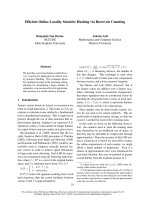
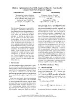
Figure 1: (a) An example of a lattice, where the
letters {A, B, C, D, E, F, G, H} represent labels
associated with nodes. (b) The degenerate lattice.
the perceptron algorithm is presented in Section 4.
3.1 Degenerate lattice
We begin by introducing the degenerate lattice,
which plays a central role in our algorithm. Con-
sider the lattice in Figure 1(a). Following conven-
tion, we regard each path on the lattice as a label
sequence. Note that the label set is {A, B, C, D,
E, F, G, H}. By aggregating several nodes in the
same column of the lattice, we can transform the
original lattice into a simpler form, which we call
the degenerate lattice (Figure 1(b)).
Let us examine the intuition behind the degen-
erate lattice. Aggregating nodes can be viewed as
grouping several labels into a new one. Here, a
label is referred to as an active label if it is not ag-
gregated (e.g., A, B, C, and D in the first column
of Figure 1(b)), and otherwise as an inactive label
(i.e., dotted nodes). The new label, which is made
by grouping the inactive labels, is referred to as

a degenerate label (i.e., large nodes covering the
dotted ones). Two degenerate labels can be seen
as equivalent if their corresponding inactive label
sets are the same (e.g., degenerate labels in the first
and the last column). In this approach, each path
of the degenerate lattice can also be interpreted as
a label sequence. In this case, however, the label to
be assigned is either an active label or a degenerate
label.
We then define the parameters associated with
degenerate label z. For reasons that will become
clear later, they are set to the maxima among the
parameters of the inactive labels:
log p(x|z)= max
y

∈I(z)
log p(x|y

), (1)
log p(z|y)= max
y

∈I(z)
log p(y

|y), (2)
log p(y|z)= max
y


∈I(z)
log p(y|y

), (3)
log p(z|z

)= max
y

∈I(z),y

∈I(z

)
log p(y

|y

), (4)
487
A A A A
B B B B
C
D
C
D
C
D
C
D

D
E
D
E
D
E
D
E
E
F
E
F
E
F
E
F
G G G G
H H H H
(a)
A
B
C
D
A A
B
A
B
C
D
(b)

Figure 2: (a) The path y = {A, E, G, C} of the
original lattice. (b) The path z of the degenerate
lattice that corresponds to y.
where y is an active label, z and z

are degenerate
labels, and I(z) denotes one-to-one mapping from
z to its corresponding inactive label set.
The degenerate lattice has an important prop-
erty which is the key to our algorithm:
Lemma 1. If the best path of the degenerate lat-
tice does not include any degenerate label, it is
equivalent to the best path of the original lattice.
Proof. Let z
max
be the best path of the degenerate
lattice. Our goal is to prove that if z
max
does not
include any degenerate label, then
∀y ∈ Y, log p(x, y) ≤ log p(x, z
max
) (5)
where Y is the set of all paths on the original lat-
tice. We prove this by partitioning Y into two dis-
joint sets: Y
0
and Y
1
, where Y

0
is the subset of
Y appearing in the degenerate lattice. Notice that
z
max
∈ Y
0
. Since z
max
is the best path of the
degenerate lattice, we have
∀y ∈ Y
0
, log p(x, y) ≤ log p(x, z
max
).
The equation holds when y = z
max
.Wenextex-
amine the label sequence y such that y ∈ Y
1
.For
each path y ∈ Y
1
, there exists a unique path z on
the degenerate lattice that corresponds to y (Fig-
ure 2). Therefore, we have
∀y ∈ Y
1
, ∃z ∈ Z, log p(x, y) ≤ log p(x, z)

< log p(x, z
max
)
where Z is the set of all paths of the degenerate
lattice. The inequality log p(x, y) ≤ log p(x, z)
can be proved by using Equations (1)-(4). Using
these results, we can complete (5).
A A A A
(a)
A A
B
A
B
A
BB
(b)
A A
B
C
D
A
B
A
B
C
D
B
C
D
C

D
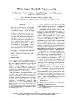
(c)
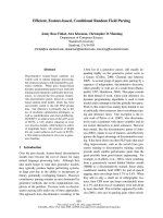
Figure 3: (a) The best path of the initial degenerate
lattice, which is denoted by the line, is located. (b)
The active labels are expanded and the best path is
searched again. (c) The best path without degen-
erate labels is obtained.
3.2 Staggered decoding
Now we can describe our algorithm, which we call
staggered decoding. The algorithm successively
constructs degenerate lattices and checks whether
the best path includes degenerate labels. In build-
ing each degenerate lattice, labels with high prob-
ability p(y), estimated from training data, are pref-
erentially selected as the active label; the expecta-
tion is that such labels are likely to belong to the
best path. The algorithm is detailed as follows:
Initialization step The algorithm starts by build-
ing a degenerate lattice in which there is only
one active label in each column. We select la-
bel y with the highest p(y) as the active label.
Search step The best path of the degenerate lat-
tice is located (Figure 3(a)). This is done
by using the Viterbi algorithm (and pruning
technique, as we describe in Section 3.3). If
the best path does not include any degenerate
label, we can terminate the algorithm since it
is identical with the best path of the original
lattice according to Lemma 1. Otherwise, we
proceed to the next step.

Expansion step We double the number of the ac-
tive labels in the degenerate lattice. The new
active labels are selected from the current in-
active label set in descending order of p(y).
If the inactive label set becomes empty, we
simply reconstructed the original lattice. Af-
ter expanding the active labels, we go back to
the previous step (Figure 3(b)). This proce-
dure is repeated until the termination condi-
tion in the search step is satisfied, i.e., the best
path has no degenerate label (Figure 3(c)).
Compared to the Viterbi algorithm, staggered
decoding requires two additional computations for
488
training. First, we have to estimate p(y) so as to
select active labels in the initialization and expan-
sion step. Second, we have to compute the pa-
rameters regarding degenerate labels according to
Equations (1)-(4). Both impose trivial computa-
tion costs.
3.3 Pruning
To achieve speed-up, it is crucial that staggered
decoding efficiently performs the search step. For
this purpose, we can basically use the Viterbi algo-
rithm. In earlier iterations, the Viterbi algorithm is
indeed efficient because the label set to be han-
dled is much smaller than the original one. In later
iterations, however, our algorithm drastically in-
creases the number of labels, making Viterbi de-
coding quite expensive.

To handle this problem, we propose a method of
pruning the lattice nodes. This technique is moti-
vated by the observation that the degenerate lattice
shares many active labels with the previous itera-
tion. In the remainder of Section3.3, we explain
the technique by taking the following steps:
• Section 3.3.1 examines a lower bound l such
that l ≤ max
y
log p(x, y).
• Section 3.3.2 examines the maximum score
M
AX(y
n
) in case token x
n
takes label y
n
:
M
AX(y
n
)= max
y

n
=y
n
log p(x, y


).
• Section 3.3.3 presents our pruning procedure.
The idea is that if M
AX(y
n
) <l, then the
node corresponding to y
n
can be removed
from consideration.
3.3.1 Lower bound
Lower bound l can be trivially calculated in the
search step. This can be done by retaining the
best path among those consisting of only active
labels. The score of that path is obviously the
lower bound. Since the search step is repeated un-
til the termination criteria is met, we can update
the lower bound at every search step. As the it-
eration proceeds, the degenerate lattice becomes
closer to the original one, so the lower bound be-
comes tighter.
3.3.2 Maximum score
The maximum score M
AX(y
n
) can be computed
from the original lattice. Let ω(y
n
) be the best
score of the partial label sequence ending with y

n
.
Presuming that we traverse the lattice from left to
right, ω(y
n
) can be defined as
max
y
n−1
{ω(y
n−1
)+logp(y
n
|y
n−1
)} +logp(x
n
|y
n
).
If we traverse the lattice from right to left, an anal-
ogous score ¯ω(y
n
) can be defined as
log p(x
n
|y
n
)+max
y

n+1
{¯ω(y
n+1
)+logp(y
n
|y
n+1
)}.
Using these two scores, we have
M
AX(y
n
)=ω(y
n
)+¯ω(y
n
) − log p(x
n
|y
n
).
Notice that updating ω(y
n
) or ¯ω(y
n
) is equivalent
to the forward or backward Viterbi algorithm, re-
spectively.
Although it is expensive to compute ω(y
n

) and
¯ω(y
n
), we can efficiently estimate their upper
bounds. Let λ(y
n
) and
¯
λ(y
n
) be scores analogous
to ω(y
n
) and ¯ω(y
n
) that are computed using the
degenerate lattice. We have ω(y
n
) ≤ λ(y
n
) and
¯ω(y
n
) ≤
¯
λ(y
n
), by following similar discussions
as raised in the proof of Lemma 1. Therefore, we
can still check whether M

AX(y
n
) is smaller than l
by using λ(y
n
) and
¯
λ(y
n
):
M
AX(y
n
)= ω(y
n
)+¯ω(y
n
) − log p(x
n
|y
n
)
≤ λ(y
n
)+
¯
λ(y
n
) − log p(x
n

|y
n
)
<l.
For the sake of simplicity, we assume that y
n
is an
active label. Although we do not discuss the other
cases, our pruning technique is also applicable to
them. We just point out that, if y
n
is an inactive
label, then there exists a degenerate label z
n
in the
n-th column such that y
n
∈ I(z
n
), and we can use
λ(z
n
) and
¯
λ(z
n
) instead of λ(y
n
) and
¯

λ(y
n
).
We compute λ(y
n
) and
¯
λ(y
n
) by using the
forward and backward Viterbi algorithm, respec-
tively. In the search step immediately following
initialization, we perform the forward Viterbi al-
gorithm to find the best path, that is, λ(y
n
) is
updated for all y
n
. In the next search step, the
backward Viterbi algorithm is carried out, and
¯
λ(y
n
) is updated. In the succeeding search steps,
these updates are alternated. As the algorithm pro-
gresses, λ(y
n
) and
¯
λ(y

n
) become closer to ω(y
n
)
and ¯ω(y
n
).
3.3.3 Pruning procedure
We make use of the bounds in pruning the lattice
nodes. To do this, we keep the values of l, λ(y
n
)
489
and
¯
λ(y
n
). They are set as l = −∞ and λ(y
n
) =
¯
λ(y
n
) = ∞ in the initialization step, and are up-
dated in the search step. The lower bound l is up-
dated at the end of the search step, while λ(y
n
)
and
¯

λ(y
n
) can be updated during the running of
the Viterbi algorithm. When λ(y
n
) or
¯
λ(y
n
) is
changed, we check whether M
AX(y
n
) <lholds
and the node is pruned if the condition is met.
3.4 Analysis
We provide here a theoretical analysis of staggered
decoding. In the following proofs, L, V , and N
represent the number of original labels, the num-
ber of distinct tokens, and the length of input token
sequence, respectively. To simplify the discussion,
we assume that log
2
L is an integer (e.g., L =64).
We first introduce three lemmas:
Lemma 2. Staggered decoding requires at most
(log
2
L +1)iterations to terminate.
Proof. We have 2

m−1
active labels in the m-th
search step (m =1, 2 ), which means we have
L active labels and no degenerate labels in the
(log
2
L +1)-th search step. Therefore, the algo-
rithm always terminates within (log
2
L +1)itera-
tions.
Lemma 3. The number of degenerate labels is
log
2
L.
Proof. Since we create one new degenerate label
in all but the last expansion step, we have log
2
L
degenerate labels.
Lemma 4. The Viterbi algorithm requires O(L
2
+
LV ) memory space and has O(NL
2
) time com-
plexity.
Proof. Since we need O(L
2
) and O(LV ) space to

keep the transition and emission probability ma-
trices, we need O(L
2
+ LV ) space to perform
the Viterbi algorithm. The time complexity of the
Viterbi algorithm is O(NL
2
) since there are NL
nodes in the lattice and it takes O(L) time to eval-
uate the score of each node.
The above statements allow us to establish our
main results:
Theorem 1. Stagger ed decoding requires O(L
2
+
LV ) memory space.
Proof. Since we have L original labels and log
2
L
degenerate labels, staggered decoding requires
O((L+log
2
L)
2
+(L+log
2
L)V )=O(L
2
+LV )
A A A A

(a)
A A
B
A
B
A
B
(b)
A A
B
C
D
A
B
A
B
C
D
(c)
Figure 4: Staggered decoding with column-wise
expansion: (a) The best path of the initial degen-
erate lattice, which does not pass through the de-
generate label in the first column. (b) Column-
wise expansion is performed and the best path is
searched again. Notice that the active label in the
first column is not expanded. (c) The final result.
memory space to perform Viterbi decoding in the
search step.
Theorem 2. Staggered decoding has O(N ) best
case time complexity and O(NL

2
) worst case time
complexity.
Proof. To perform the m-th search step, staggered
decoding requires the order of O(N4
m−1
) time
because we have 2
m−1
active labels. Therefore, it
has O(

M
m=1
N4
m−1
) time complexity if it termi-
nates after the M-th search step. In the best case,
M =1, the time complexity is O(N). In the worst
case, M =log
2
L +1, the time complexity is the
order of O(NL
2
) because

log
2
L+1
m=1

N4
m−1
<
4
3
NL
2
.
Theorem 1 shows that staggered decoding
asymptotically requires the same order of mem-
ory space as the Viterbi algorithm. Theorem 2 re-
veals that staggered decoding has the same order
of time complexity as the Viterbi algorithm even
in the worst case.
3.5 Heuristic techniques
We present two heuristic techniques for further
speeding up our algorithm.
First, we can initialize the value of lower bound
l by selecting a path from the original lattice in
some way, and then computing the score of that
path. In our experiments, we use the path lo-
cated by the left-to-right deterministic decoding
(i.e., beam search with a beam width of 1). Al-
though this method requires an additional cost to
locate the path, it is very effective in practice. If
l is initialized in this manner, the best case time
complexity of our algorithm becomes O(NL).
490
The second technique is for the expansion step.
Instead of the expansion technique described in

Section 3.2, we can expand the active labels in a
heuristic manner to keep the number of active la-
bels small:
Column-wise expansion step We double the
number of the active labels in the column
only if the best path of the degenerate lattice
passes through the degenerate label of that
column (Figure 4).
A drawback of this strategy is that the algorithm
requires N(log
2
L+1) iterations in the worst case.
As the result, we can no longer derive a reasonable
upper bound for the time complexity. Neverthe-
less, column-wise expansion is highly effective in
practice as we will demonstrate in the experiment.
Note that Theorem 1 still holds true even if we use
column-wise expansion.
4 Extension to the Perceptron
The discussion we have made so far can be applied
to perceptrons. This can be clarified by comparing
the score functions f(x, y). In HMMs, the score
function can be written as
N

n=1

log(x
n
|y

n
)+log(y
n
|y
n−1
)

.
In perceptrons, on the other hand, it is given as
N

n=1


k
w
1
k
φ
1
k
(x,y
n
)+

k
w
2
k
φ

2
k
(x,y
n−1
,y
n
)

where we explicitly distinguish the unigram fea-
ture function φ
1
k
and bigram feature function φ
2
k
.
Comparing the form of the two functions, we can
see that our discussion on HMMs can be extended
to perceptrons by substituting

k
w
1
k
φ
1
k
(x,y
n
)

and

k
w
2
k
φ
2
k
(x,y
n−1
,y
n
) for log p(x
n
|y
n
) and
log p(y
n
|y
n−1
).
However, implementing the perceptron algo-
rithm is not straightforward. The problem is
that it is difficult, if not impossible, to compute

k
w
1

k
φ
1
k
(x,y) and

k
w
2
k
φ
2
k
(x,y,y

) offline be-
cause they are dependent on the entire token se-
quence x, unlike log p(x|y) and log p(y|y

). Con-
sequently, we cannot evaluate the maxima analo-
gous to Equations (1)-(4) offline either.
For unigram features, we compute the maxi-
mum, max
y

k
w
1
k

φ
1
k
(x,y), as a preprocess in
the initialization step (cf. Equation (1)). This pre-
process requires O(NL) time, which is negligible
compared with the cost required by the Viterbi al-
gorithm.
Unfortunately, we cannot use the same tech-
nique for computing max
y,y


k
w
2
k
φ
2
k
(x,y,y

)
because a similar computation would take
O(NL
2
) time (cf. Equation (4)). For bigram fea-
tures, we compute its upper bound offline. For ex-
ample, the following bound was proposed by Es-
posito and Radicioni (2009):

max
y,y


k
w
2
k
φ
2
k
(x,y,y

) ≤ max
y,y


k
w
2
k
δ(0 <w
2
k
)
where δ(·) is the delta function and the summa-
tions are taken over all feature functions associated
with both y and y

. Intuitively, the upper bound

corresponds to an ideal case in which all features
with positive weight are activated.
3
It can be com-
puted without any task-specific knowledge.
In practice, however, we can compute better
bounds based on task-specific knowledge. The
simplest case is that the bigram features are inde-
pendent of the token sequence x. In such a situ-
ation, we can trivially compute the exact maxima
offline, as we did in the case of HMMs. Fortu-
nately, such a feature set is quite common in NLP
problems and we could use this technique in our
experiments. Even if bigram features are depen-
dent on x, it is still possible to compute better
bounds if several features are mutually exclusive,
as discussed in (Esposito and Radicioni, 2009).
Finally, it is worth noting that we can use stag-
gered decoding in training perceptrons as well, al-
though such application lies outside the scope of
this paper. The algorithm does not support train-
ing acceleration for other discriminative models.
5 Experiments and Discussion
5.1 Setting
The proposed algorithm was evaluated with three
tasks: POS tagging, joint POS tagging and chunk-
ing (called joint tagging for short), and supertag-
ging. To reduce joint tagging into a single se-
quence labeling problem, we produced the labels
by concatenating the POS tag and the chunk tag

(BIO format), e.g., NN/B-NP. In the two tasks
other than supertagging, the input token is the
word. In supertagging, the token is the pair of the
word and its oracle POS tag.
3
We assume binary feature functions.
491
Table 1: Decoding speed (sent./sec).
POS tagging Joint tagging Supertagging
VITERBI 4000 77 1.1
CARPEDIEM 8600 51 0.26
SD 8800 850 121
SD+C-EXP. 14,000 1600 300
The data sets we used for the three experiments
are the Penn TreeBank (PTB) corpus, CoNLL
2000 corpus, and an HPSG treebank built from the
PTB corpus (Matsuzaki et al., 2007). We used sec-
tions 02-21 of PTB for training, and section 23 for
testing. The number of labels in the three tasks is
45, 319 and 2602, respectively.
We used the perceptron algorithm for train-
ing. The models were averaged over 10 itera-
tions (Collins, 2002). For features, we basically
followed previous studies (Tsuruoka and Tsujii,
2005; Sha and Pereira, 2003; Ninomiya et al.,
2006). In POS tagging, we used unigrams of the
current and its neighboring words, word bigrams,
prefixes and suffixes of the current word, capital-
ization, and tag bigrams. In joint tagging, we also
used the same features. In supertagging, we used

POS unigrams and bigrams in addition to the same
features other than capitalization.
As the evaluation measure, we used the average
decoding speed (sentences/sec) to two significant
digits over five trials. To strictly measure the time
spent for decoding, we ignored the preprocessing
time, that is, the time for loading the model file
and converting the features (i.e., strings) into inte-
gers. We note that the accuracy was comparable to
the state-of-the-art in the three tasks: 97.08, 93.21,
and 91.20% respectively.
5.2 Results and discussions
Table 1 presents the performance of our algo-
rithm. SD represents the proposed algorithm with-
out column-wise expansion, while SD+
C-EXP.
uses column-wise expansion. For comparison, we
present the results of two baseline algorithms as
well: V
ITERBI and CARPEDIEM (Esposito and
Radicioni, 2009). In almost all settings, we see
that both of our algorithms outperformed the other
two. We also find that SD+
C-EXP. performed con-
sistently better than SD. This indicates the effec-
tiveness of column-wise expansion.
Following V
ITERBI,CARPEDIEM is the most
relevant algorithm, for sequence labeling in NLP,
as discussed in Section 2.3. However, our results

Table 2: The average number of iterations.
POS tagging Joint tagging Supertagging
SD 6.02 8.15 10.0
SD+C-EXP. 6.12 8.62 10.6
Table 3: Training time.
POS tagging Joint tagging Supertagging
VITERBI 100 sec. 20 min. 100 hour
SD+C-EXP. 37 sec. 1.5 min. 5.3 hour
demonstrated that CARPEDIEM worked poorly in
two of the three tasks. We consider this is because
the transition information is crucial for the two
tasks, and the assumption behind C
ARPEDIEM is
violated. In contrast, the proposed algorithms per-
formed reasonably well for all three tasks, demon-
strating the wide applicability of our algorithm.
Table 2 presents the average iteration num-
bers of SD and SD+
C-EXP. We can observe
that the two algorithms required almost the same
number of iterations on average, although the
iteration number is not tightly bounded if we
use column-wise expansion. This indicates that
SD+
C-EXP. virtually avoided performing extra it-
erations, while heuristically restricting active label
expansion.
Table 3 compares the training time spent by
V
ITERBI and SD+C-EXP. Although speeding up

perceptron training is a by-product, it is interest-
ing to see that our algorithm is in fact effective at
reducing the training time as well. The result also
indicates that the speed-up is more significant at
test time. This is probably because the model is
not predictive enough at the beginning of training,
and the pruning is not that effective.
5.3 Comparison with approximate algorithm
Table 4 compares two exact algorithms (V
ITERBI
and SD+E-XP.) with beam search, which is the ap-
proximate algorithm widely adopted for sequence
labeling in NLP. For this experiment, the beam
width, B, was exhaustively calibrated: we tried B
= {1, 2, 4, 8, } until the beam search achieved
comparable accuracy to the exact algorithms, i.e.,
the difference fell below 0.1 in our case.
We see that there is a substantial difference in
the performance between V
ITERBI and BEAM.
On the other hand, SD+
C-EXP. reached speeds
very close to those of B
EAM. In fact, they
achieved comparable performance in our exper-
iment. These results demonstrate that we could
successfully bridge the gap in the performance be-
492
Table 4: Comparison with beam search (sent./sec).
POS tagging Joint tagging Supertagging

VITERBI 4000 77 1.1
SD+C-EXP. 14,000 1600 300
BEAM 18,000 2400 180
tween exact and approximate algorithms, while re-
taining the advantages of exact algorithms.
6 Relation to coarse-to-fine approach
Before concluding remarks, we briefly examine
the relationship between staggered decoding and
coarse-to-fine PCFG parsing (2006). In coarse-to-
fine parsing, the candidate parse trees are pruned
by using the parse forest produced by a coarse-
grained PCFG. Since the degenerate label can be
interpreted as a coarse-level label, one may con-
sider that staggered decoding is an instance of
coarse-to-fine approach. While there is some re-
semblance, there are at least two essential differ-
ences. First, coarse-to-fine approach is a heuristic
pruning, that is, it is not an exact algorithm. Sec-
ond, our algorithm does not always perform de-
coding at the fine-grained level. It is designed to
be able to stop decoding at the coarse-level.
7 Conclusions
The sequence labeling algorithm is indispensable
to modern statistical NLP. However, the Viterbi
algorithm, which is the standard decoding algo-
rithm in NLP, is not efficient when we have to
deal with a large number of labels. In this paper
we presented staggered decoding, which provides
a principled way of resolving this problem. We
consider that it is a real alternative to the Viterbi

algorithm in various NLP tasks.
An interesting future direction is to extend the
proposed technique to handle more complex struc-
tures than the Markov chains, including semi-
Markov models and factorial HMMs (Sarawagi
and Cohen, 2004; Sutton et al., 2004). We hope
this work opens a new perspective on decoding al-
gorithms for a wide range of NLP problems, not
just sequence labeling.
Acknowledgement
We wish to thank the anonymous reviewers for
their helpful comments, especially on the com-
putational complexity of our algorithm. We also
thank Yusuke Miyao for providing us with the
HPSG Treebank data.
References
Thorsten Brants. 2000. TnT - a statistical part-of-
speech tagger. In Proceedings of ANLP, pages 224–
231.
Eugene Charniak, MarkJohnson, Micha Elsner, Joseph
Austerweil, David Ellis, Isaac Haxton, Catherine
Hill, R. Shrivaths, Jeremy Moore, Michael Pozar,
and Theresa Vu. 2006. Multi-level coarse-to-fine
PCFG parsing. In Proceedings of NAACL, pages
168–175.
Trevor Cohn. 2006. Efficient inference in large con-
ditional random fields. In Proceedings of ECML,
pages 606–613.
Michael Collins. 2002. Discriminative training meth-
ods for hidden Markov models: Theory and exper-

iments with perceptron algorithms. In Proceedings
of EMNLP, pages 1–8.
Thomas G. Dietterich, Pedro Domingos, Lise Getoor,
Stephen Muggleton, and Prasad Tadepalli. 2008.
Structured machine learning: the next ten years.
Machine Learning, 73(1):3–23.
Roberto Esposito and Daniele P. Radicioni. 2009.
C
ARPEDIEM: Optimizing the Viterbi algorithm
and applications to supervised sequential learning.
Jorunal of Machine Learning Research, 10:1851–
1880.
Pedro F. Felzenszwalb, Daniel P. Huttenlocher, and
Jon M. Kleinberg. 2003. Fast algorithms for large-
state-space HMMs with applications to Web usage
analysis. In Proceedings of NIPS, pages 409–416.
Minwoo Jeong, Chin-Yew Lin, and Gary Geunbae Lee.
2009. Efficient inference of CRFs for large-scale
natural language data. In Proceedings of ACL-
IJCNLP Short Papers, pages 281–284.
John Lafferty, Andrew McCallum, and Fernand
Pereira. 2001. Conditional random fields: Prob-
abilistic models for segmenting and labeling se-
quence data. In Proceedings of ICML, pages 282–
289.
Percy Liang, Hal Daum´e III, and Dan Klein. 2008.
Structure compilation: Trading structure for fea-
tures. In Proceedings of ICML, pages 592–599.
YuryLifshits, Shay Mozes, OrenWeimann, and Michal
Ziv-Ukelson. 2007. Speeding up HMM decod-

ing and training by exploiting sequence repetitions.
Computational Pattern Matching, pages 4–15.
Dekang Lin and Xiaoyun Wu. 2009. Phrae clustering
for discriminative training. In Proceedings of ACL-
IJCNLP, pages 1030–1038.
493
Takuya Matsuzaki, Yusuke Miyao, and Jun’ichi Tsu-
jii. 2007. Efficient HPSG parsing with supertagging
and CFG-filtering. In Proceedings of IJCAI, pages
1671–1676.
Takashi Ninomiya, Takuya Matsuzaki, Yoshimasa Tsu-
ruoka, Yusuke Miyao, and Jun’ichi Tsujii. 2006.
Extremely lexicalized models for accurate and fast
HPSG parsing. In Proceedings of EMNLP, pages
155–163.
Lawrence R. Rabiner. 1989. A tutorial on hidden
Markov models and selected applications in speech
recognition. In Proceedings of The IEEE, pages
257–286.
Sunita Sarawagi and Willian W. Cohen. 2004. Semi-
Markov conditional random fields for information
extraction. In Proceedings of NIPS, pages 1185–
1192.
Fei Sha and Fernando Pereira. 2003. Shallow parsing
with conditional random fields. In Proceedings of
HLT-NAACL, pages 134–141.
Sajid M. Siddiqi and Andrew W. Moore. 2005. Fast
inference and learning in large-state-space HMMs.
In Proceedings of ICML, pages 800–807.
Charles Sutton, Khashayar Rohanimanesh, and An-

drew McCallum. 2004. Dynamic conditional ran-
dom fields: Factorized probabilistic models for la-
beling and segmenting sequence data. In Proceed-
ings of ICML.
Ben Tasker, Carlos Guestrin, and Daphe Koller. 2003.
Max-margin Markov networks. In Proceedings of
NIPS, pages 25–32.
Ioannis Tsochantaridis, Thorsten Joachims, Thomas
Hofmann, and Yasemin Altun. 2005. Large margin
methods for structured and interdependent output
variables. Journal of Machine Learning Research,
6:1453–1484.
Yoshimasa Tsuruoka and Jun’ichi Tsujii. 2005. Bidi-
rectional inference with the easiest-first strategy
for tagging sequence data. In Proceedings of
HLT/EMNLP, pages 467–474.
Andrew J. Viterbi. 1967. Error bounds for convo-
lutional codes and an asymeptotically optimum de-
coding algorithm. IEEE Transactios on Information
Theory, 13(2):260–267.
494