Báo cáo khoa học: "Semisupervised condensed nearest neighbor for part-of-speech tagging" pot
Bạn đang xem bản rút gọn của tài liệu. Xem và tải ngay bản đầy đủ của tài liệu tại đây (142.45 KB, 5 trang )
Proceedings of the 49th Annual Meeting of the Association for Computational Linguistics:shortpapers, pages 48–52,
Portland, Oregon, June 19-24, 2011.
c
2011 Association for Computational Linguistics
Semisupervised condensed nearest neighbor for part-of-speech tagging
Anders Søgaard
Center for Language Technology
University of Copenhagen
Njalsgade 142, DK-2300 Copenhagen S
Abstract
This paper introduces a new training set con-
densation technique designed for mixtures
of labeled and unlabeled data. It finds a
condensed set of labeled and unlabeled data
points, typically smaller than what is obtained
using condensed nearest neighbor on the la-
beled data only, and improves classification
accuracy. We evaluate the algorithm on semi-
supervised part-of-speech tagging and present
the best published result on the Wall Street
Journal data set.
1 Introduction
Labeled data for natural language processing tasks
such as part-of-speech tagging is often in short sup-
ply. Semi-supervised learning algorithms are de-
signed to learn from a mixture of labeled and un-
labeled data. Many different semi-supervised algo-
rithms have been applied to natural language pro-
cessing tasks, but the simplest algorithm, namely
self-training, is the one that has attracted most atten-
tion, together with expectation maximization (Ab-
ney, 2008). The idea behind self-training is simply
to let a model trained on the labeled data label the
unlabeled data points and then to retrain the model
on the mixture of the original labeled data and the
newly labeled data.
The nearest neighbor algorithm (Cover and Hart,
1967) is a memory-based or so-called lazy learn-
ing algorithm. It is one of the most extensively
used nonparametric classification algorithms, sim-
ple to implement yet powerful, owing to its theo-
retical properties guaranteeing that for all distribu-
tions, its probability of error is bound by twice the
Bayes probability of error (Cover and Hart, 1967).
Memory-based learning has been applied to a wide
range of natural language processing tasks including
part-of-speech tagging (Daelemans et al., 1996), de-
pendency parsing (Nivre, 2003) and word sense dis-
ambiguation (K¨ubler and Zhekova, 2009). Memory-
based learning algorithms are said to be lazy be-
cause no model is learned from the labeled data
points. The labeled data points are the model. Con-
sequently, classification time is proportional to the
number of labeled data points. This is of course im-
practical. Many algorithms have been proposed to
make memory-based learning more efficient. The
intuition behind many of them is that the set of la-
beled data points can be reduced or condensed, since
many labeled data points are more or less redundant.
The algorithms try to extract a subset of the overall
training set that correctly classifies all the discarded
data points through the nearest neighbor rule. Intu-
itively, the model finds good representatives of clus-
ters in the data or discards the data points that are far
from the decision boundaries. Such algorithms are
called training set condensation algorithms.
The need for training set condensation is partic-
ularly important in semi-supervised learning where
we rely on a mixture of labeled and unlabeled data
points. While the number of labeled data points
is typically limited, the number of unlabeled data
points is typically high. In this paper, we intro-
duce a new semi-supervised learning algorithm that
combines self-training and condensation to produce
small subsets of labeled and unlabeled data points
that are highly relevant for determining good deci-
48
sion boundaries.
2 Semi-supervised condensed nearest
neighbor
The nearest neighbor (NN) algorithm (Cover and
Hart, 1967) is conceptually simple, yet very pow-
erful. Given a set of labeled data points T , label any
new data point (feature vector) x with y where x
′
is the data point in T most similar to x and x
′
, y.
Similarity is usually measured in terms of Euclidean
distance. The generalization of the nearest neighbor
algorithm, k nearest neighbor, finds the k most simi-
lar data points T
k
to x and assigns x the label ˆy such
that:
ˆy = arg max
y
′′
∈Y
Σ
x
′
,y
′
∈T
k
E(x, x
′
)||y
′
= y
′′
||
with E(·, ·) Euclidean distance and || · || = 1 if the
argument is true (else 0). In other words, the k most
similar points take a weighted vote on the class of x.
Naive implementations of the algorithm store all
the labeled data points and compare each of them to
the data point that is to be classified. Several strate-
gies have been proposed to make nearest neighbor
classification more efficient (Angiulli, 2005). In
particular, training set condensation techniques have
been much studied.
The condensed nearest neighbor (CNN) algorithm
was first introduced in Hart (1968). Finding a sub-
set of the labeled data points may lead to faster
and more accurate classification, but finding the best
subset is an intractable problem (Wilfong, 1992).
CNN can be seen as a simple technique for approxi-
mating such a subset of labeled data points.
The CNN algorithm is defined in Figure 1 with T
the set of labeled data points and T (t) is label pre-
dicted for t by a nearest neighbor classifier ”trained”
on T .
Essentially we discard all labeled data points
whose label we can already predict with the cur-
rent subset of labeled data points. Note that we
have simplified the CNN algorithm a bit compared
to Hart (1968), as suggested, for example, in Alpay-
din (1997), iterating only once over data rather than
waiting for convergence. This will give us a smaller
set of labeled data points, and therefore classifica-
tion requires less space and time. Note that while
the NN rule is stable, and cannot be improved by
T = {x
1
, y
1
, . . . , x
n
, y
n
}, C = ∅
for x
i
, y
i
∈ T do
if C(x
i
) = y
i
then
C = C ∪ {x
i
, y
i
}
end if
end for
return C
Figure 1: CONDENSED NEAREST NEIGHBOR.
T = {x
1
, y
1
, . . . , x
n
, y
n
}, C = ∅
for x
i
, y
i
∈ T do
if C(x
i
) = y
i
or P
C
(x
i
, y
i
|x
i
) < 0.55 then
C = C ∪ {x
i
, y
i
}
end if
end for
return C
Figure 2: WEAKENED CONDENSED NEAREST NEIGH-
BOR.
techniques such as bagging (Breiman, 1996), CNN
is unstable (Alpaydin, 1997).
We also introduce a weakened version of the al-
gorithm which not only includes misclassified data
points in the classifier C, but also correctly classi-
fied data points which were labeled with relatively
low confidence. So C includes all data points that
were misclassified and those whose correct label
was predicted with low confidence. The weakened
condensed nearest neighbor (WCNN) algorithm is
sketched in Figure 2.
C inspects k nearest neighbors when labeling
new data points, where k is estimated by cross-
validation. CNN was first generalized to k-NN in
Gates (1972).
Two related condensation techniques, namely re-
moving typical elements and removing elements by
class prediction strength, were argued not to be
useful for most problems in natural language pro-
cessing in Daelemans et al. (1999), but our experi-
ments showed that CNN often perform about as well
as NN, and our semi-supervised CNN algorithm
leads to substantial improvements. The condensa-
tion techniques are also very different: While re-
moving typical elements and removing elements by
class prediction strength are methods for removing
data points close to decision boundaries, CNN ide-
49
Figure 3: Unlabeled data may help find better representa-
tives in condensed training sets.
ally only removes elements close to decision bound-
aries when the classifier has no use of them.
Intuitively, with relatively simple problems,
e.g. mixtures of Gaussians, CNN and WCNN try to
find the best possible representatives for each clus-
ter in the distribution of data, i.e. finding the points
closest to the center of each cluster. Ideally, CNN
returns one point for each cluster, namely the cen-
ter of each cluster. However, a sample of labeled
data may not include data points that are near the
center of a cluster. Consequently, CNN sometimes
needs several points to stabilize the representation of
a cluster; e.g. the two positives in Figure 3.
When a large number of unlabeled data points
that are labeled according to nearest neighbors pop-
ulates the clusters, chances increase that we find data
points near the centers of our clusters, e.g. the ”good
representative” in Figure 3. Of course the centers of
our clusters may move, but the positive results ob-
tained experimentally below suggest that it is more
likely that labeling unlabeled data by nearest neigh-
bors will enable us to do better training set conden-
sation.
This is exactly what semi-supervised condensed
nearest neighbor (SCNN) does. We first run a
WCNN C and obtain a condensed set of labeled data
points. To this set of labeled data points we add a
large number of unlabeled data points labeled by a
NN classifier T on the original data set. We use a
simple selection criterion and include all data points
1: T = {x
1
, y
1
, . . . , x
n
, y
n
}, C = ∅, C
′
= ∅
2: U = {x
′
1
, . . . , x
′
m
} # unlabeled data
3: for x
i
, y
i
∈ T do
4: if C(x
i
) = y
i
or P
C
(x
i
, y
i
|x
i
) < 0.55
then
5: C = C ∪ {x
i
, y
i
}
6: end if
7: end for
8: for x
′
i
∈ U do
9: if P
T
(x
′
i
, T (x
′
i
)|w
i
) > 0.90 then
10: C = C ∪ {x
′
i
, T (x
′
i
)}
11: end if
12: end for
13: for x
i
, y
i
∈ C do
14: if C
′
(x
i
) = y
i
then
15: C
′
= C
′
∪ {x
i
, y
i
}
16: end if
17: end for
18: return C
′
Figure 4: SEMI-SUPERVISED CONDENSED NEAREST
NEIGHBOR.
that are labeled with confidence greater than 90%.
We then obtain a new WCNN C
′
from the new data
set which is a mixture of labeled and unlabeled data
points. See Figure 4 for details.
3 Part-of-speech tagging
Our part-of-speech tagging data set is the standard
data set from Wall Street Journal included in Penn-
III (Marcus et al., 1993). We use the standard splits
and construct our data set in the following way, fol-
lowing Søgaard (2010): Each word in the data w
i
is associated with a feature vector x
i
= x
1
i
, x
2
i
where x
1
i
is the prediction on w
i
of a supervised part-
of-speech tagger, in our case SVMTool
1
(Gimenez
and Marquez, 2004) trained on Sect. 0–18, and x
2
i
is a prediction on w
i
from an unsupervised part-of-
speech tagger (a cluster label), in our case Unsu-
pos (Biemann, 2006) trained on the British National
Corpus.
2
We train a semi-supervised condensed
nearest neighbor classifier on Sect. 19 of the devel-
opment data and unlabeled data from the Brown cor-
pus and apply it to Sect. 22–24. The labeled data
1
/>2
/>50
points are thus of the form (one data point or word
per line):
JJ JJ 17*
NNS NNS 1
IN IN 428
DT DT 425
where the first column is the class labels or the
gold tags, the second column the predicted tags and
the third column is the ”tags” provided by the unsu-
pervised tagger. Words marked by ”*” are out-of-
vocabulary words, i.e. words that did not occur in
the British National Corpus. The unsupervised tag-
ger is used to cluster tokens in a meaningful way.
Intuitively, we try to learn part-of-speech tagging by
learning when to rely on SVMTool.
The best reported results in the literature on Wall
Street Journal Sect. 22–24 are 97.40% in Suzuki et
al. (2009) and 97.44% in Spoustova et al. (2009);
both systems use semi-supervised learning tech-
niques. Our semi-supervised condensed nearest
neighbor classifier achieves an accuracy of 97.50%.
Equally importantly it condensates the available data
points, from Sect. 19 and the Brown corpus, that
is more than 1.2M data points, to only 2249 data
points, making the classifier very fast. CNN alone is
a lot worse than the input tagger, with an accuracy
of 95.79%. Our approach is also significantly better
than Søgaard (2010) who apply tri-training (Li and
Zhou, 2005) to the output of SVMTool and Unsu-
pos.
acc (%) data points err.red
CNN 95.79 3,811
SCNN
97.50 2,249 40.6%
SVMTool 97.15 -
Søgaard 97.27 -
Suzuki et al. 97.40 -
Spoustova et al.
97.44 -
In our second experiment, where we vary the
amount of unlabeled data points, we only train our
ensemble on the first 5000 words in Sect. 19 and
evaluate on the first 5000 words in Sect. 22–24.
The derived learning curve for the semi-supervised
learner is depicted in Figure 5. The immediate drop
in the red scatter plot illustrates the condensation ef-
fect of semi-supervised learning: when we begin to
add unlabeled data, accuracy increases by more than
1.5% and the data set becomes more condensed.
Semi-supervised learning means that we populate
Figure 5: Normalized accuracy (range: 92.62–94.82) and
condensation (range: 310–512 data points).
clusters in the data, making it easier to identify rep-
resentative data points. Since we can easier identify
representative data points, training set condensation
becomes more effective.
4 Implementation
The implementation used in the experiments builds
on Orange 2.0b for Mac OS X (Python and C++).
In particular, we made use of the implementations
of Euclidean distance and random sampling in their
package. Our code is available at:
cst.dk/anders/sccn/
5 Conclusions
We have introduced a new learning algorithm that
simultaneously condensates labeled data and learns
from a mixture of labeled and unlabeled data. We
have compared the algorithm to condensed nearest
neighbor (Hart, 1968; Alpaydin, 1997) and showed
that the algorithm leads to more condensed models,
and that it performs significantly better than con-
densed nearest neighbor. For part-of-speech tag-
ging, the error reduction over condensed nearest
neighbor is more than 40%, and our model is 40%
smaller than the one induced by condensed nearest
neighbor. While we have provided no theory for
semi-supervised condensed nearest neighbor, we be-
lieve that these results demonstrate the potential of
the proposed method.
51
References
Steven Abney. 2008. Semi-supervised learning for com-
putational linguistics. Chapman & Hall.
Ethem Alpaydin. 1997. Voting over multiple con-
densed nearest neighbors. Artificial Intelligence Re-
view, 11:115–132.
Fabrizio Angiulli. 2005. Fast condensed nearest neigh-
bor rule. In Proceedings of the 22nd International
Conference on Machine Learning.
Chris Biemann. 2006. Unsupervised part-of-speech
tagging employing efficient graph clustering. In
COLING-ACL Student Session.
Leo Breiman. 1996. Bagging predictors. Machine
Learning, 24(2):123–140.
T. Cover and P. Hart. 1967. Nearest neighbor pattern
classification. IEEE Transactions on Information The-
ory, 13(1):21–27.
Walter Daelemans, Jakub Zavrel, Peter Berck, and Steven
Gillis. 1996. MBT: a memory-based part-of-speech
tagger generator. In Proceedings of the 4th Workshop
on Very Large Corpora.
Walter Daelemans, Antal Van Den Bosch, and Jakub Za-
vrel. 1999. Forgetting exceptions is harmful in lan-
guage learning. Machine Learning, 34(1–3):11–41.
W Gates. 1972. The reduced nearest neighbor rule.
IEEE Transactions on Information Theory, 18(3):431–
433.
Jesus Gimenez and Lluis Marquez. 2004. SVMTool: a
general POS tagger generator based on support vector
machines. In LREC.
Peter Hart. 1968. The condensed nearest neighbor rule.
IEEE Transactions on Information Theory, 14:515–
516.
Sandra K¨ubler and Desislava Zhekova. 2009. Semi-
supervised learning for word-sense disambiguation:
quality vs. quantity. In RANLP.
Ming Li and Zhi-Hua Zhou. 2005. Tri-training: ex-
ploiting unlabeled data using three classifiers. IEEE
Transactions on Knowledge and Data Engineering,
17(11):1529–1541.
Mitchell Marcus, Mary Marcinkiewicz, and Beatrice
Santorini. 1993. Building a large annotated corpus
of English: the Penn Treebank. Computational Lin-
guistics, 19(2):313–330.
Joakim Nivre. 2003. An efficient algorithm for projec-
tive dependency parsing. In Proceedings of the 8th In-
ternational Workshop on Parsing Technologies, pages
149–160.
Anders Søgaard. 2010. Simple semi-supervised training
of part-of-speech taggers. In ACL.
Drahomira Spoustova, Jan Hajic, Jan Raab, and Miroslav
Spousta. 2009. Semi-supervised training for the aver-
aged perceptron POS tagger. In EACL.
Jun Suzuki, Hideki Isozaki, Xavier Carreras, and Michael
Collins. 2009. An empirical study of semi-supervised
structured conditional models for dependency parsing.
In EMNLP.
G. Wilfong. 1992. Nearest neighbor problems. Interna-
tional Journal of Computational Geometry and Appli-
cations, 2(4):383–416.
52