Báo cáo khoa học: "Semi-Supervised Cause Identification from Aviation Safety Reports" pot
Bạn đang xem bản rút gọn của tài liệu. Xem và tải ngay bản đầy đủ của tài liệu tại đây (171.16 KB, 9 trang )
Proceedings of the 47th Annual Meeting of the ACL and the 4th IJCNLP of the AFNLP, pages 843–851,
Suntec, Singapore, 2-7 August 2009.
c
2009 ACL and AFNLP
Semi-Supervised Cause Identification from Aviation Safety Reports
Isaac Persing and Vincent Ng
Human Language Technology Research Institute
University of Texas at Dallas
Richardson, TX 75083-0688
{persingq,vince}@hlt.utdallas.edu
Abstract
We introduce cause identification, a new
problem involving classification of in-
cident reports in the aviation domain.
Specifically, given a set of pre-defined
causes, a cause identification system seeks
to identify all and only those causes that
can explain why the aviation incident de-
scribed in a given report occurred. The dif-
ficulty of cause identification stems in part
from the fact that it is a multi-class, multi-
label categorization task, and in part from
the skewness of the class distributions and
the scarcity of annotated reports. To im-
prove the performance of a cause identi-
fication system for the minority classes,
we present a bootstrapping algorithm that
automatically augments a training set by
learning from a small amount of labeled
data and a large amount of unlabeled data.
Experimental results show that our algo-
rithm yields a relative error reduction of
6.3% in F-measure for the minority classes
in comparison to a baseline that learns
solely from the labeled data.
1 Introduction
Automatic text classification is one of the most im-
portant applications in natural language process-
ing (NLP). The difficulty of a text classification
task depends on various factors, but typically, the
task can be difficult if (1) the amount of labeled
data available for learning the task is small; (2)
it involves multiple classes; (3) it involves multi-
label categorization, where more than one label
can be assigned to each document; (4) the class
distributions are skewed, with some categories
significantly outnumbering the others; and (5) the
documents belong to the same domain (e.g., movie
review classification). In particular, when the doc-
uments to be classified are from the same domain,
they tend to be more similar to each other with
respect to word usage, thus making the classes
less easily separable. This is one of the reasons
why topic-based classification, even with multiple
classes as in the 20 Newsgroups dataset
1
, tends to
be easier than review classification, where reviews
from the same domain are to be classified accord-
ing to the sentiment expressed
2
.
In this paper, we introduce a new text classifi-
cation problem involving the Aviation Safety Re-
porting System (ASRS) that can be viewed as a
difficult task along each of the five dimensions dis-
cussed above. Established in 1967, ASRS collects
voluntarily submitted reports about aviation safety
incidents written by flight crews, attendants, con-
trollers, and other related parties. These incident
reports are made publicly available to researchers
for automatic analysis, with the ultimate goal of
improving the aviation safety situation. One cen-
tral task in the automatic analysis of these reports
is cause identification, or the identification of why
an incident happened. Aviation safety experts at
NASA have identified 14 causes (or shaping fac-
tors in NASA terminology) that could explain why
an incident occurred. Hence, cause identification
can be naturally recast as a text classification task:
given an incident report, determine which of a set
of 14 shapers contributed to the occurrence of the
incident described in the report.
As mentioned above, cause identification is
considered challenging along each of the five
aforementioned dimensions. First, there is a
scarcity of incident reports labeled with the
shapers. This can be attributed to the fact that
there has been very little work on this task. While
the NASA researchers have applied a heuristic
method for labeling a report with shapers (Posse
1
/>2
Of course, the fact that sentiment classification requires
a deeper understanding of a text also makes it more difficult
than topic-based text classification (Pang et al., 2002).
843
et al., 2005), the method was evaluated on only
20 manually labeled reports, which are not made
publicly available. Second, the fact that this is
a 14-class classification problem makes it more
challenging than a binary classification problem.
Third, a report can be labeled with more than one
category, as several shapers can contribute to the
occurrence of an aviation incident. Fourth, the
class distribution is very skewed: based on an
analysis of our 1,333 annotated reports, 10 of the
14 categories can be considered minority classes,
which account for only 26% of the total num-
ber of labels associated with the reports. Finally,
our cause identification task is domain-specific,
involving the classification of documents that all
belong to the aviation domain.
This paper focuses on improving the accuracy
of minority class prediction for cause identifica-
tion. Not surprisingly, when trained on a dataset
with a skewed class distribution, most supervised
machine learning algorithms will exhibit good per-
formance on the majority classes, but relatively
poor performance on the minority classes. Unfor-
tunately, achieving good accuracies on the minor-
ity classes is very important in our task of identify-
ing shapers from aviation safety reports, where 10
out of the 14 shapers are minority classes, as men-
tioned above. Minority class prediction has been
tackled extensively in the machine learning liter-
ature, using methods that typically involve sam-
pling and re-weighting of training instances, with
the goal of creating a less skewed class distribution
(e.g., Pazzani et al. (1994), Fawcett (1996), Ku-
bat and Matwin (1997)). Such methods, however,
are unlikely to perform equally well for our cause
identification task given our small labeled set, as
the minority class prediction problem is compli-
cated by the scarcity of labeled data. More specif-
ically, given the scarcity of labeled data, many
words that are potentially correlated with a shaper
(especially a minority shaper) may not appear in
the training set, and the lack of such useful indi-
cators could hamper the acquisition of an accurate
classifier via supervised learning techniques.
We propose to address the problem of minority
class prediction in the presence of a small training
set by means of a bootstrapping approach, where
we introduce an iterative algorithm to (1) use a
small set of labeled reports and a large set of unla-
beled reports to automatically identify words that
are most relevant to the minority shaper under con-
sideration, and (2) augment the labeled data by us-
ing the resulting words to annotate those unlabeled
reports that can be confidently labeled. We evalu-
ate our approach using cross-validation on 1,333
manually annotated reports. In comparison to a
supervised baseline approach where a classifier is
acquired solely based on the training set, our boot-
strapping approach yields a relative error reduc-
tion of 6.3% in F-measure for the minority classes.
In sum, the contributions of our work are three-
fold. First, we introduce a new, challenging
text classification problem, cause identification
from aviation safety reports, to the NLP commu-
nity. Second, we created an annotated dataset for
cause identification that is made publicly available
for stimulating further research on this problem
3
.
Third, we introduce a bootstrapping algorithm for
improving the prediction of minority classes in the
presence of a small training set.
The rest of the paper is organized as follows. In
Section 2, we present the 14 shapers. Section 3 ex-
plains how we preprocess and annotate the reports.
Sections 4 and 5 describe the baseline approaches
and our bootstrapping algorithm, respectively. We
present results in Section 6, discuss related work
in Section 7, and conclude in Section 8.
2 Shaping Factors
As mentioned in the introduction, the task of cause
identification involves labeling an incident report
with all the shaping factors that contributed to the
occurrence of the incident. Table 1 lists the 14
shaping factors, as well as a description of each
shaper taken verbatim from Posse et al. (2005).
As we can see, the 14 classes are not mutually ex-
clusive. For instance, a lack of familiarity with
equipment often implies a deficit in proficiency in
its use, so the two shapers frequently co-occur. In
addition, while some classes cover a specific and
well-defined set of issues (e.g., Illusion), some en-
compass a relatively large range of situations. For
instance, resource deficiency can include prob-
lems with equipment, charts, or even aviation per-
sonnel. Furthermore, ten shaping factors can be
considered minority classes, as each of them ac-
count for less than 10% of the labels. Accurately
predicting minority classes is important in this do-
main because, for example, the physical factors
minority shaper is frequently associated with in-
cidents involving near-misses between aircraft.
3
/>844
Id Shaping Factor Description %
1 Attitude Any indication of unprofessional or antagonistic attitude by a controller or flight crew mem-
ber, e.g., complacency or get-homeitis (in a hurry to get home).
2.4
2 Communication
Environment
Interferences with communications in the cockpit such as noise, auditory interference, radio
frequency congestion, or language barrier.
5.5
3 Duty Cycle A strong indication of an unusual working period, e.g., a long day, flying very late at night,
exceeding duty time regulations, having short and inadequate rest periods.
1.8
4 Familiarity A lack of factual knowledge, such as new to or unfamiliar with company, airport, or aircraft. 3.2
5 Illusion Bright lights that cause something to blend in, black hole, white out, sloping terrain, etc. 0.1
6 Other Anything else that could be a shaper, such as shift change, passenger discomfort, or disori-
entation.
13.3
7 Physical
Environment
Unusual physical conditions that could impair flying or make things difficult. 16.0
8 Physical
Factors
Pilot ailment that could impair flying or make things more difficult, such as being tired,
drugged, incapacitated, suffering from vertigo, illness, dizziness, hypoxia, nausea, loss of
sight or hearing.
2.2
9 Preoccupation A preoccupation, distraction, or division of attention that creates a deficit in performance,
such as being preoccupied, busy (doing something else), or distracted.
6.7
10 Pressure Psychological pressure, such as feeling intimidated, pressured, or being low on fuel. 1.8
11 Proficiency A general deficit in capabilities, such as inexperience, lack of training, not qualified, or not
current.
14.4
12 Resource
Deficiency
Absence, insufficient number, or poor quality of a resource, such as overworked or unavail-
able controller, insufficient or out-of-date chart, malfunctioning or inoperative or missing
equipment.
30.0
13 Taskload Indicators of a heavy workload or many tasks at once, such as short-handed crew. 1.9
14 Unexpected Something sudden and surprising that is not expected. 0.6
Table 1: Descriptions of shaping factor classes. The “%” column shows the percent of labels the shapers account for.
3 Dataset
We downloaded our corpus from the ASRS web-
site
4
. The corpus consists of 140,599 incident
reports collected during the period from January
1998 to December 2007. Each report is a free
text narrative that describes not only why an in-
cident happened, but also what happened, where it
happened, how the reporter felt about the incident,
the reporter’s opinions of other people involved in
the incident, and any other comments the reporter
cared to include. In other words, a lot of informa-
tion in the report is irrelevant to (and thus compli-
cates) the task of cause identification.
3.1 Preprocessing
Unlike newswire articles, at which many topic-
based text classification tasks are targeted, the
ASRS reports are informally written using various
domain-specific abbreviations and acronyms, tend
to contain poor grammar, and have capitalization
information removed, as illustrated in the follow-
ing sentence taken from one of the reports.
HAD BEEN CLRED FOR APCH BY
ZOA AND HAD BEEN HANDED OFF
TO SANTA ROSA TWR.
4
/>This sentence is grammatically incorrect (due to
the lack of a subject), and contains abbrevia-
tions such as CLRED, APCH, and TWR. This
makes it difficult for a non-aviation expert to un-
derstand. To improve readability (and hence fa-
cilitate the annotation process), we preprocess
each report as follows. First, we expand the ab-
breviations/acronyms with the help of an official
list of acronyms/abbreviations and their expanded
forms
5
. Second, though not as crucial as the first
step, we heuristically restore the case of the words
by relying on an English lexicon: if a word ap-
pears in the lexicon, we assume that it is not a
proper name, and therefore convert it into lower-
case. After preprocessing, the example sentence
appears as
had been cleared for approach by ZOA
and had been handed off to santa rosa
tower.
Finally, to facilitate automatic analysis, we stem
each word in the narratives.
3.2 Human Annotation
Next, we randomly picked 1,333 preprocessed re-
ports and had two graduate students not affiliated
5
See />ASRS
Decode.pdf. In the very infrequently-occurring case
where the same abbreviation or acronym may have more
than expansion, we arbitrarily chose one of the possibilities.
845
Id Total (%) F1 F2 F3 F4 F5
1 52 (3.9) 11 7 7 17 10
2 119 (8.9) 29 29 22 16 23
3 38 (2.9) 10 5 6 9 8
4 70 (5.3) 11 12 9 14 24
5 3 (0.2) 0 0 0 1 2
6 289 (21.7) 76 44 60 42 67
7 348 (26.1) 73 63 82 59 71
8 48 (3.6) 11 14 8 11 4
9 145 (10.9) 29 25 38 28 25
10 38 (2.9) 12 10 4 7 5
11 313 (23.5) 65 50 74 46 78
12 652 (48.9) 149 144 125 123 111
13 42 (3.2) 7 8 8 6 13
14 14 (1.1) 3 3 3 3 2
Table 2: Number of occurrences of each shaping
factor in the dataset. The “Total” column shows the num-
ber of narratives labeled with each shaper and the percentage
of narratives tagged with each shaper in the 1,333 labeled
narrative set. The “F” columns show the number narratives
associated with each shaper in folds F1 – F5.
x (# Shapers) 1 2 3 4 5 6
Percentage 53.6 33.2 10.3 2.7 0.2 0.1
Table 3: Percentage of documents with x labels.
with this research independently annotate them
with shaping factors, based solely on the defi-
nitions presented in Table 1. To measure inter-
annotator agreement, we compute Cohen’s Kappa
(Carletta, 1996) from the two sets of annotations,
obtaining a Kappa value of only 0.43. This not
only suggests the difficulty of the cause identifica-
tion task, but also reveals the vagueness inherent
in the definition of the 14 shapers. As a result,
we had the two annotators re-examine each report
for which there was a disagreement and reach an
agreement on its final set of labels. Statistics of the
annotated dataset can be found in Table 2, where
the “Total” column shows the size of each of the
14 classes, expressed both as the number of re-
ports that are labeled with a particular shaper and
as a percent (in parenthesis). Since we will per-
form 5-fold cross validation in our experiments,
we also show the number of reports labeled with
each shaper under the “F” columns for each fold.
To get a better idea of how many reports have mul-
tiple labels, we categorize the reports according to
the number of labels they contain in Table 3.
4 Baseline Approaches
In this section, we describe two baseline ap-
proaches to cause identification. Since our ulti-
mate goal is to evaluate the effectiveness of our
bootstrapping algorithm, the baseline approaches
only make use of small amounts of labeled data for
acquiring classifiers. More specifically, both base-
lines recast the cause identification problem as a
set of 14 binary classification problems, one for
predicting each shaper. In the binary classification
problem for predicting shaper s
i
, we create one
training instance from each document in the train-
ing set, labeling the instance as positive if the doc-
ument has s
i
as one of its labels, and negative oth-
erwise. After creating training instances, we train
a binary classifier, c
i
, for predicting s
i
, employing
as features the top 50 unigrams that are selected
according to information gain computed over the
training data (see Yang and Pedersen (1997)). The
SVM learning algorithm as implemented in the
LIBSVM software package (Chang and Lin, 2001)
is used for classifier training, owing to its robust
performance on many text classification tasks.
In our first baseline, we set all the learning pa-
rameters to their default values. As noted before,
we divide the 1,333 annotated reports into five
folds of roughly equal size, training the classifiers
on four folds and applying them separately to the
remaining fold. Results are reported in terms of
precision (P), recall (R), and F-measure (F), which
are computed by aggregating over the 14 shapers
as follows. Let tp
i
be the number of test reports
correctly labeled as positive by c
i
; p
i
be the total
number of test reports labeled as positive by c
i
;
and n
i
be the total number of test reports that be-
long to s
i
according to the gold standard. Then,
P =
i
tp
i
i
p
i
, R =
i
tp
i
i
n
i
, and F =
2P R
P + R
.
Our second baseline is similar to the first, ex-
cept that we tune the classification threshold (CT)
to optimize F-measure. More specifically, recall
that LIBSVM trains a classifier that by default em-
ploys a CT of 0.5, thus classifying an instance as
positive if and only if the probability that it be-
longs to the positive class is at least 0.5. How-
ever, this may not be the optimal threshold to use
as far as performance is concerned, especially for
the minority classes, where the class distribution
is skewed. This is the motivation behind tuning
the CT of each classifier. To ensure a fair compar-
ison with the first baseline, we do not employ ad-
ditional labeled data for parameter tuning; rather,
we reserve 25% of the available training data for
tuning, and use the remaining 75% for classifier
846
acquisition. This amounts to using three folds
for training and one fold for development in each
cross validation experiment. Using the develop-
ment data, we tune the 14 CTs jointly to optimize
overall F-measure. However, an exact solution to
this optimization problem is computationally ex-
pensive. Consequently, we find a local maximum
by employing a local search algorithm, which al-
ters one parameter at a time to optimize F-measure
by holding the remaining parameters fixed.
5 Our Bootstrapping Algorithm
One of the potential weaknesses of the two base-
lines described in the previous section is that the
classifiers are trained on only a small amount of
labeled data. This could have an adverse effect
on the accuracy of the resulting classifiers, espe-
cially those for the minority classes. The situation
is somewhat aggravated by the fact that we are
adopting a one-versus-all scheme for generating
training instances for a particular shaper, which,
together with the small amount of labeled data, im-
plies that only a couple of positive instances may
be available for training the classifier for a minor-
ity class. To alleviate the data scarcity problem
and improve the accuracy of the classifiers, we
propose in this section a bootstrapping algorithm
that automatically augments a training set by ex-
ploiting a large amount of unlabeled data. The ba-
sic idea behind the algorithm is to iteratively iden-
tify words that are high-quality indicators of the
positive or negative examples, and then automati-
cally label unlabeled documents that contain a suf-
ficient number of such indicators.
Our bootstrapping algorithm, shown in Figure
1, aims to augment the set of positive and neg-
ative training instances for a given shaper. The
main function, Train, takes as input four argu-
ments. The first two arguments, P and N , are the
positive and negative instances, respectively, gen-
erated by the one-versus-one scheme from the ini-
tial training set, as described in the previous sec-
tion. The third argument, U , is the unlabeled set
of documents, which consists of all but the doc-
uments in the training set. In particular, U con-
tains the documents in the development and test
sets. Hence, we are essentially assuming access
to the test documents (but not their labels) dur-
ing the training process, as in a transductive learn-
ing setting. The last argument, k, is the number
of bootstrapping iterations. In addition, the algo-
T rain(P, N, U, k)
Inputs:
P : positively labeled training examples of shaper x
N: negatively labeled training examples of shaper x
U: set of unlabeled narratives in corpus
k: number of bootstrapping iterations
P W ← ∅
NW ← ∅
for i = 0 to k − 1 do
if |P | > |N | then
[P, P W ] ← ExpandT rainingSet(P, N, U, PW )
else
[N, NW ] ←ExpandT rainingSet(N,P, U, NW )
end if
end for
ExpandT rainingSet(A, B, U, W )
Inputs:
A, B, U: narrative sets
W : unigram feature set
for j = 1 to 4 do
t ← arg max
t /∈W
log(
C(t,A)
C(t,B)+1
)
// C(t, X): number of narratives in X containing t
W ← W ∪ {t}
end for
return [A ∪ S(W, U ), W ]
// S(W, U ): narratives in U containing ≥ 3 words in W
Figure 1: Our bootstrapping algorithm.
rithm uses two variables, P W and N W , to store
the sets of high-quality indicators for the positive
instances and the negative instances, respectively,
that are found during the bootstrapping process.
Next, we begin our k bootstrapping iterations.
In each iteration, we expand either P or N , de-
pending on their relative sizes. In order to keep
the two sets as close in size as possible, we choose
to expand the smaller of the two sets.
6
After that,
we execute the function ExpandTrainingSet to ex-
pand the selected set. Without loss of general-
ity, assume that P is chosen for expansion. To
do this, ExpandTrainingSet selects four words that
seem much more likely to appear in P than in
N from the set of candidate words
7
. To select
these words, we calculate the log likelihood ratio
log(
C(t,P )
C(t,N)+1
) for each candidate word t, where
C(t, P ) is the number of narratives in P that con-
tain t, and C(t, N) similarly is the number of nar-
ratives in N that contain t. If this ratio is large,
6
It may seem from the way P and N are constructed that
N is almost always larger than P and therefore is unlikely to
be selected for expansion. However, the ample size of the un-
labeled set means that the algorithm still adds large numbers
of narratives to the training data. Hence, even for minority
classes, P often grows larger than N by iteration 3.
7
A candidate word is a word that appears in the training
set (P ∪ N) at least four times.
847
we posit that t is a good indicator of P . Note that
incrementing the count in the denominator by one
has a smoothing effect: it avoids selecting words
that appears infrequently in P and not at all in N .
There is a reason for selecting multiple words
(rather than just one word) in each bootstrap-
ping iteration: we want to prevent the algorithm
from selecting words that are too specific to one
subcategory of a shaping factor. For example,
shaping factor 7 (Physical Environment) is com-
posed largely of incidents influenced by weather
phenomena. In one experiment, we tried select-
ing only one word per bootstrapping iteration.
For shaper 7, the first word added to PW was
“snow”. Upon the next iteration, the algorithm
added “plow” to PW. While “plow” may itself be
indicative of shaper 7, we believe its selection was
due to the recent addition to P of a large number of
narratives containing “snow”. Hence, by selecting
four words per iteration, we are forcing the algo-
rithm to “branch out” among these subcategories.
After adding the selected words to P W , we
augment P with all the unlabeled documents con-
taining at least three words from P W . The rea-
son we impose the “at least three” requirement
is precision: we want to ensure, with a reason-
able level of confidence, that the unlabeled doc-
uments chosen to augment P should indeed be
labeled with the shaper under consideration, as
incorrectly labeled documents would contaminate
the labeled data, thus accelerating the deterioration
of the quality of the automatically labeled data in
subsequent bootstrapping iterations and adversely
affecting the accuracy of the classifier trained on it
(Pierce and Cardie, 2001).
The above procedure is repeated in each boot-
strapping iteration. As mentioned above, if N
is smaller in size than P , we will expand N in-
stead, adding to N W the four words that are the
strongest indicators of a narrative being a negative
example of the shaper under consideration, and
augmenting N with those unlabeled narratives that
contain at least three words from NW .
The number of bootstrapping iterations is con-
trolled by the input parameter k. As we will see
in the next section, we run the bootstrapping algo-
rithm for up to five iterations only, as the quality
of the bootstrapped data deteriorates fairly rapidly.
The exact value of k will be determined automati-
cally using development data, as discussed below.
After bootstrapping, the augmented training
data can be used in combination with any of the
two baseline approaches to acquire a classifier for
identifying a particular shaper. Whichever base-
line is used, we need to reserve one of the five
folds to tune the parameter k in our cross vali-
dation experiments. In particular, if the second
baseline is used, we will tune CT and k jointly
on the development data using the local search al-
gorithm described previously, where we adjust the
values of both CT and k for one of the 14 classi-
fiers in each step of the search process to optimize
the overall F-measure score.
6 Evaluation
6.1 Baseline Systems
Since our evaluation centers on the question of
how effective our bootstrapping algorithm is in ex-
ploiting unlabeled documents to improve classifier
performance, our two baselines only employ the
available labeled documents to train the classifiers.
Recall that our first baseline, which we call
B
0.5
(due to its being a baseline with a CT of
0.5), employs default values for all of the learn-
ing parameters. Micro-averaged 5-fold cross val-
idation results of this baseline for all 14 shapers
and for just 10 minority classes (due to our focus
on improving minority class prediction) are ex-
pressed as percentages in terms of precision (P),
recall (R), and F-measure (F) in the first row of
Table 4. As we can see, the baseline achieves
an F-measure of 45.4 (14 shapers) and 35.4 (10
shapers). Comparing these two results, the higher
F-measure achieved using all 14 shapers can be at-
tributed primarily to improvements in recall. This
should not be surprising: as mentioned above, the
number of positive instances of a minority class
may be small, thus causing the resulting classi-
fier to be biased towards classifying a document
as negative.
Instead of employing a CT value of 0.5, our
second baseline, B
ct
, tunes CT using one of the
training folds and simply trains a classifier on the
remaining three folds. For parameter tuning, we
tested CTs of 0.0, 0.05, . . ., 1.0. Results of this
baseline are shown in row 2 of Table 4. In com-
parison to the first baseline, we see that F-measure
improves considerably by 7.4% and 4.5% for 14
shapers and 10 shapers respectively
8
, which illus-
8
It is important to note that the parameters are optimized
separately for each pair of 14-shaper and 10-shaper exper-
iments in this paper, and that the 10-shaper results are not
848
All 14 Classes 10 Minority Classes
System P R F P R F
B
0.5
67.0 34.4 45.4 68.3 23.9 35.4
B
ct
47.4 59.2 52.7 47.8 34.3 39.9
E
0.5
60.9 40.4 48.6 53.2 35.3 42.4
E
ct
50.5 54.9 52.6 49.1 39.4 43.7
Table 4: 5-fold cross validation results.
trates the importance of employing the right CT
for the cause identification task.
6.2 Our Approach
Next, we evaluate the effectiveness of our boot-
strapping algorithm in improving classifier per-
formance. More specifically, we apply the two
baselines separately to the augmented training set
produced by our bootstrapping algorithm. When
combining our bootstrapping algorithm with the
first baseline, we produce a system that we call
E
0.5
(due to its being trained on the expanded
training set with a CT of 0.5). E
0.5
has only one
tunable parameter, k (i.e., the number of boot-
strapping iterations), whose allowable values are
0, 1, . . ., 5. When our algorithm is used in com-
bination with the second baseline, we produce an-
other system, E
ct
, which has both k and the CT
as its parameters. The allowable values of these
parameters, which are to be tuned jointly, are the
same as those employed by B
ct
and E
0.5
.
Results of E
0.5
are shown in row 3 of Table
4. In comparison to B
0.5
, we see that F-measure
increases by 3.2% and 7.0% for 14 shapers and
10 shapers, respectively. Such increases can be
attributed to less imbalanced recall and precision
values, as a result of a large gain in recall accom-
panied by a roughly equal drop in precision. These
results are consistent with our intuition: recall can
be improved with a larger training set, but preci-
sion can be hampered when learning from nois-
ily labeled data. Overall, these results suggest that
learning from the augmented training set is useful,
especially for the minority classes.
Results of E
ct
are shown in row 4 of Table 4.
In comparison to B
ct
, we see mixed results: F-
measure increases by 3.8% for 10 shapers (which
represents a relative error reduction of 6.3%, but
drops by 0.1% for 14 shapers. Overall, these re-
sults suggest that when the CT is tunable, train-
ing set expansion helps the minority classes but
hurts the remaining classes. A closer look at the
results reveals that the 0.1% F-measure drop is due
simply extracted from the 14-shaper experiments.
to a large drop in recall accompanied by a smaller
gain in precision. In other words, for the four
non-minority classes, the benefits obtained from
using the bootstrapped documents can also be ob-
tained by simply adjusting the CT. This could be
attributed to the fact that a decent classifier can be
trained using only the hand-labeled training exam-
ples for these four shapers, and as a result, the au-
tomatically labeled examples either provide very
little new knowledge or are too noisy to be useful.
On the other hand, for the 10 minority classes, the
3.8% gain in F-measure can be attributed to a si-
multaneous rise in recall and precision. Note that
such gain cannot possibly be obtained by simply
adjusting the CT, since adjusting the CT always
results in higher recall and lower precision or vice
versa. Overall, the simultaneous rise in recall and
precision implies that the bootstrapped documents
have provided useful knowledge, particularly in
the form of positive examples, for the classifiers.
Even though the bootstrapped documents are nois-
ily labeled, they can still be used to improve the
classifiers, as the set of initially labeled positive
examples for the minority classes is too small.
6.3 Additional Analyses
Quality of the bootstrapped data. Since the
bootstrapped documents are noisily labeled, a nat-
ural question is: How noisy are they? To get a
sense of the accuracy of the bootstrapped docu-
ments without further manual labeling, recall that
our experimental setup resembles a transductive
setting where the test documents are part of the
unlabeled data, and consequently, some of them
may have been automatically labeled by the boot-
strapping algorithm. In fact, 137 documents in the
five test folds were automatically labeled in the
14-shaper E
ct
experiments, and 69 automatically
labeled documents were similarity obtained from
the 10-shaper E
ct
experiments. For 14 shapers, the
accuracies of the positively and negatively labeled
documents are 74.6% and 97.1%, respectively,
and the corresponding numbers for 10 shapers are
43.2% and 81.3%. These numbers suggest that
negative examples can be acquired with high ac-
curacies, but the same is not true for positive ex-
amples. Nevertheless, learning the 10 shapers
from the not-so-accurately-labeled positive exam-
ples still allows us to outperform the correspond-
ing baseline.
849
Shaping Factor Positive Expanders Negative Expanders
Familiarity unfamiliar, layout, unfamilarity, rely
Physical Environment cloud, snow, ice, wind
Physical Factors fatigue, tire, night, rest, hotel, awake, sleep, sick declare, emergency, advisory, separation
Preoccupation distract, preoccupied, awareness, situational,
task, interrupt, focus, eye, configure, sleep
declare, ice snow, crash, fire, rescue, anti,
smoke
Pressure bad, decision, extend, fuel, calculate, reserve,
diversion, alternate
Table 5: Example positive and negative expansion words collected by E
ct
for selected shaping factors.
Analysis of the expanders. To get an idea of
whether the words acquired during the bootstrap-
ping process (henceforth expanders) make intu-
itive sense, we show in Table 5 example positive
and negative expanders obtained for five shaping
factors from the E
ct
experiments. As we can see,
many of the positive expanders are intuitively ob-
vious. We might, however, wonder about the con-
nection between, for example, the shaper Famil-
iarity and the word “rely”, or between the shaper
Pressure and the word “extend”. We suspect that
the bootstrapping algorithm is likely to make poor
word selections particularly in the cases of the mi-
nority classes, where the positively labeled train-
ing data used to select expansion words is more
sparse. As suggested earlier, poor word choice
early in the algorithm is likely to cause even poorer
word choice later on.
On the other hand, while none of the negative
expanders seem directly meaningful in relation to
the shaper for which they were selected, some of
them do appear to be related to other phenomena
that may be negatively correlated with the shaper.
For instance, the words “snow” and “ice” were
selected as negative expanders for Preoccupation
and also as positive expanders for Physical Envi-
ronment. While these two shapers are only slightly
negatively correlated, it is possible that Preoccu-
pation may be strongly negatively correlated with
the subset of Physical Environment incidents in-
volving cold weather.
7 Related Work
Since we recast cause identification as a text clas-
sification task and proposed a bootstrapping ap-
proach that targets at improving minority class
prediction, the work most related to ours involves
one or both of these topics.
Guzm´an-Cabrera et al. (2007) address the
problem of class skewness in text classification.
Specifically, they first under-sample the majority
classes, and then bootstrap the classifier trained
on the under-sampled data using unlabeled doc-
uments collected from the Web.
Minority classes can be expanded without the
availability of unlabeled data as well. For ex-
ample, Chawla et al. (2002) describe a method
by which synthetic training examples of minor-
ity classes can be generated from other labeled
training examples to address the problem of im-
balanced data in a variety of domains.
Nigam et al. (2000) propose an iterative semi-
supervised method that employs the EM algorithm
in combination with the naive Bayes generative
model to combine a small set of labeled docu-
ments and a large set of unlabeled documents. Mc-
Callum and Nigam (1999) suggest that the ini-
tial labeled examples can be obtained using a list
of keywords rather than through annotated data,
yielding an unsupervised algorithm.
Similar bootstrapping methods are applicable
outside text classification as well. One of the
most notable examples is Yarowsky’s (1995) boot-
strapping algorithm for word sense disambigua-
tion. Beginning with a list of unlabeled contexts
surrounding a word to be disambiguated and a list
of seed words for each possible sense, the algo-
rithm iteratively uses the seeds to label a training
set from the unlabeled contexts, and then uses the
training set to identify more seed words.
8 Conclusions
We have introduced a new problem, cause identi-
fication from aviation safety reports, to the NLP
community. We recast it as a multi-class, multi-
label text classification task, and presented a boot-
strapping algorithm for improving the prediction
of minority classes in the presence of a small train-
ing set. Experimental results show that our algo-
rithm yields a relative error reduction of 6.3% in
F-measure over a purely supervised baseline when
applied to the minority classes. By making our
annotated dataset publicly available, we hope to
stimulate research in this challenging problem.
850
Acknowledgments
We thank the three anonymous reviewers for their
invaluable comments on an earlier draft of the
paper. We are indebted to Muhammad Arshad
Ul Abedin, who provided us with a preprocessed
version of the ASRS corpus and, together with
Marzia Murshed, annotated the 1,333 documents.
This work was supported in part by NASA Grant
NNX08AC35A and NSF Grant IIS-0812261.
References
Jean Carletta. 1996. Assessing agreement on classi-
fication tasks: The Kappa statistic. Computational
Linguistics, 22(2):249–254.
Chih-Chung Chang and Chih-Jen Lin, 2001. LIB-
SVM: A library for support vector machines.
Software available at .
edu.tw/
∼
cjlin/libsvm.
Nitesh V. Chawla, Kevin W. Bowyer, Lawrence O.
Hall, and W. Philip Kegelmeyer. 2002. SMOTE:
Synthetic minority over-sampling technique. Jour-
nal of Artificial Intelligence Research, 16:321–357.
Tom Fawcett. 1996. Learning with skewed class distri-
butions — summary of responses. Machine Learn-
ing List: Vol. 8, No. 20.
Rafael Guzm´an-Cabrera, Manuel Montes-y-G´omez,
Paolo Rosso, and Luis Villase˜nor Pineda. 2007.
Taking advantage of the Web for text classification
with imbalanced classes. In Proceedings of MICAI,
pages 831–838.
Miroslav Kubat and Stan Matwin. 1997. Addressing
the curse of imbalanced training sets: One-sided se-
lection. In Proceedings of ICML, pages 179–186.
Andrew McCallum and Kamal Nigam. 1999. Text
classification by bootstrapping with keywords, EM
and shrinkage. In Proceedings of the ACL Work-
shop for Unsupervised Learning in Natural Lan-
guage Processing, pages 52–58.
Kamal Nigam, Andrew McCallum, Sebastian Thrun,
and Tom Mitchell. 2000. Text classification from
labeled and unlabeled documents using EM. Ma-
chine Learning, 39(2/3):103–134.
Bo Pang, Lillian Lee, and Shivakumar Vaithyanathan.
2002. Thumbs up? Sentiment classification us-
ing machine learning techniques. In Proceedings of
EMNLP, pages 79–86.
Michael Pazzani, Christopher Merz, Patrick Murphy,
Kamal Ali, Timothy Hume, and Clifford Brunk.
1994. Reducing misclassification costs. In Proceed-
ings of ICML, pages 217–225.
David Pierce and Claire Cardie. 2001. Limitations of
co-training for natural language learning from large
datasets. In Proceedings of EMNLP, pages 1–9.
Christian Posse, Brett Matzke, Catherine Anderson,
Alan Brothers, Melissa Matzke, and Thomas Ferry-
man. 2005. Extracting information from narratives:
An application to aviation safety reports. In Pro-
ceedings of the Aerospace Conference 2005, pages
3678–3690.
Yiming Yang and Jan O. Pedersen. 1997. A compara-
tive study on feature selection in text categorization.
In Proceedings of ICML, pages 412–420.
David Yarowsky. 1995. Unsupervised word sense dis-
ambiguation rivaling supervised methods. In Pro-
ceedings of the ACL, pages 189–196.
851