Báo cáo khoa học: "Efficient, Feature-based, Conditional Random Field Parsing" potx

Proceedings of ACL-08: HLT, pages 959–967,
Columbus, Ohio, USA, June 2008.
c
2008 Association for Computational Linguistics
Efficient, Feature-based, Conditional Random Field Parsing
Jenny Rose Finkel, Alex Kleeman, Christopher D. Manning
Department of Computer Science
Stanford University
Stanford, CA 94305
jrfi, ,
Abstract
Discriminative feature-based methods are
widely used in natural language processing,
but sentence parsing is still dominated by gen-
erative methods. While prior feature-based
dynamic programming parsers have restricted
training and evaluation to artificially short sen-
tences, we present the first general, feature-
rich discriminative parser, based on a condi-
tional random field model, which has been
successfully scaled to the full WSJ parsing
data. Our efficiency is primarily due to the
use of stochastic optimization techniques, as
well as parallelization and chart prefiltering.
On WSJ15, we attain a state-of-the-art F-score
of 90.9%, a 14% relative reduction in error
over previous models, while being two orders
of magnitude faster. On sentences of length
40, our system achieves an F-score of 89.0%,
a 36% relative reduction in error over a gener-
ative baseline.

1 Introduction
Over the past decade, feature-based discriminative
models have become the tool of choice for many
natural language processing tasks. Although they
take much longer to train than generative models,
they typically produce higher performing systems,
in large part due to the ability to incorporate ar-
bitrary, potentially overlapping features. However,
constituency parsing remains an area dominated by
generative methods, due to the computational com-
plexity of the problem. Previous work on discrim-
inative parsing falls under one of three approaches.
One approach does discriminative reranking of the
n-best list of a generative parser, still usually de-
pending highly on the generative parser score as
a feature (Collins, 2000; Charniak and Johnson,
2005). A second group of papers does parsing by a
sequence of independent, discriminative decisions,
either greedily or with use of a small beam (Ratna-
parkhi, 1997; Henderson, 2004). This paper extends
the third thread of work, where joint inference via
dynamic programming algorithms is used to train
models and to attempt to find the globally best parse.
Work in this context has mainly been limited to use
of artificially short sentences due to exorbitant train-
ing and inference times. One exception is the re-
cent work of Petrov et al. (2007), who discrimina-
tively train a grammar with latent variables and do
not restrict themselves to short sentences. However
their model, like the discriminative parser of John-

son (2001), makes no use of features, and effectively
ignores the largest advantage of discriminative train-
ing. It has been shown on other NLP tasks that mod-
eling improvements, such as the switch from gen-
erative training to discriminative training, usually
provide much smaller performance gains than the
gains possible from good feature engineering. For
example, in (Lafferty et al., 2001), when switching
from a generatively trained hidden Markov model
(HMM) to a discriminatively trained, linear chain,
conditional random field (CRF) for part-of-speech
tagging, their error drops from 5.7% to 5.6%. When
they add in only a small set of orthographic fea-
tures, their CRF error rate drops considerably more
to 4.3%, and their out-of-vocabulary error rate drops
by more than half. This is further supported by John-
son (2001), who saw no parsing gains when switch-
959
ing from generative to discriminative training, and
by Petrov et al. (2007) who saw only small gains of
around 0.7% for their final model when switching
training methods.
In this work, we provide just such a framework for
training a feature-rich discriminative parser. Unlike
previous work, we do not restrict ourselves to short
sentences, but we do provide results both for training
and testing on sentences of length ≤ 15 (WSJ15) and
for training and testing on sentences of length ≤ 40,
allowing previous WSJ15 results to be put in context
with respect to most modern parsing literature. Our

model is a conditional random field based model.
For a rule application, we allow arbitrary features
to be defined over the rule categories, span and split
point indices, and the words of the sentence. It is
well known that constituent length influences parse
probability, but PCFGs cannot easily take this infor-
mation into account. Another benefit of our feature
based model is that it effortlessly allows smooth-
ing over previously unseen rules. While the rule
may be novel, it will likely contain features which
are not. Practicality comes from three sources. We
made use of stochastic optimization methods which
allow us to find optimal model parameters with very
few passes through the data. We found no differ-
ence in parser performance between using stochastic
gradient descent (SGD), and the more common, but
significantly slower, L-BFGS. We also used limited
parallelization, and prefiltering of the chart to avoid
scoring rules which cannot tile into complete parses
of the sentence. This speed-up does not come with a
performance cost; we attain an F-score of 90.9%, a
14% relative reduction in errors over previous work
on WSJ15.
2 The Model
2.1 A Conditional Random Field Context Free
Grammar (CRF-CFG)
Our parsing model is based on a conditional ran-
dom field model, however, unlike previous TreeCRF
work, e.g., (Cohn and Blunsom, 2005; Jousse et al.,
2006), we do not assume a particular tree structure,

and instead find the most likely structure and la-
beling. This is similar to conventional probabilis-
tic context-free grammar (PCFG) parsing, with two
exceptions: (a) we maximize conditional likelihood
of the parse tree, given the sentence, not joint like-
lihood of the tree and sentence; and (b) probabil-
ities are normalized globally instead of locally –
the graphical models depiction of our trees is undi-
rected.
Formally, we have a CFG G, which consists of
(Manning and Sch¨utze, 1999): (i) a set of termi-
nals {w
k
},k = 1, ,V; (ii) a set of nonterminals
{N
k
},k = 1, ,n; (iii) a designated start symbol
ROOT; and (iv) a set of rules, {
ρ
= N
i
→
ζ
j
}, where
ζ
j
is a sequence of terminals and nonterminals. A
PCFG additionally assigns probabilities to each rule
ρ

such that ∀i
∑
j
P(N
i
→
ζ
j
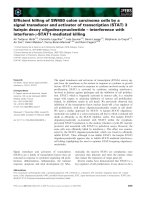
) = 1. Our conditional
random field CFG (CRF-CFG) instead defines local
clique potentials
φ
(r|s;
θ
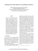
), where s is the sentence,
and r contains a one-level subtree of a tree t, corre-
sponding to a rule
ρ
, along with relevant information
about the span of words which it encompasses, and,
if applicable, the split position (see Figure 1). These
potentials are relative to the sentence, unlike a PCFG
where rule scores do not have access to words at the
leaves of the tree, or even how many words they
dominate. We then define a conditional probabil-
ity distribution over entire trees, using the standard
CRF distribution, shown in (1). There is, however,
an important subtlety lurking in how we define the
partition function. The partition function Z
s

, which
makes the probability of all possible parses sum to
unity, is defined over all structures as well as all la-
belings of those structures. We define
τ
(s) to be the
set of all possible parse trees for the given sentence
licensed by the grammar G.
P(t|s;
θ
) =
1
Z
s
∏
r∈t
φ
(r|s;
θ
) (1)
where
Z
s
=
∑
t∈
τ
(s)
∏
r∈t

′
φ
(r|s;
θ
)
The above model is not well-defined over all
CFGs. Unary rules of the form N
i
→ N
j
can form
cycles, leading to infinite unary chains with infinite
mass. However, it is standard in the parsing liter-
ature to transform grammars into a restricted class
of CFGs so as to permit efficient parsing. Binariza-
tion of rules (Earley, 1970) is necessary to obtain
cubic parsing time, and closure of unary chains is re-
quired for finding total probability mass (rather than
just best parses) (Stolcke, 1995). To address this is-
sue, we define our model over a restricted class of
960
S
NP
NN
Factory
NNS
payrolls
VP
VBD
fell

PP
IN
in
NN
September
Phrasal rules
r
1
= S
0,5
→ NP
0,2
VP
2,5
| Factory payrolls fell in September
r
3
= VP
2,5
→ VBD
2,3
PP
3,5
| Factory payrolls fell in September

Lexicon rules
r
5
= NN
0,1

→ Factory | Factory payrolls fell in September
r
6
= NNS
1,2
→ payrolls | Factory payrolls fell in September

(a) PCFG Structure (b) Rules r
Figure 1: A parse tree and the corresponding rules over which potentials and features are defined.
CFGs which limits unary chains to not have any re-
peated states. This was done by collapsing all al-
lowed unary chains to single unary rules, and dis-
allowing multiple unary rule applications over the
same span.
1
We give the details of our binarization
scheme in Section 5. Note that there exists a gram-
mar in this class which is weakly equivalent with any
arbitrary CFG.
2.2 Computing the Objective Function
Our clique potentials take an exponential form. We
have a feature function, represented by f(r,s), which
returns a vector with the value for each feature. We
denote the value of feature f
i
by f
i
(r,s) and our
model has a corresponding parameter
θ

i
for each
feature. The clique potential function is then:
φ
(r|s;
θ
) = exp
∑
i
θ
i
f
i
(r,s) (2)
The log conditional likelihood of the training data
D, with an additional L
2
regularization term, is then:
L (D;
θ
) =

∑
(t,s)∈D

∑
r∈t
∑
i
θ

i
f
i
(r,s)

− Z
s

+
∑
i
θ
2
i
2
σ
2
(3)
And the partial derivatives of the log likelihood, with
respect to the model weights are, as usual, the dif-
ference between the empirical counts and the model
expectations:
∂
L
∂θ
i
=

∑
(t,s)∈D


∑
r∈t
f
i
(r,s)

− E
θ
[ f
i
|s]

+
θ
i
σ
2
(4)
1
In our implementation of the inside-outside algorithm, we
then need to keep two inside and outside scores for each span:
one from before and one from after the application of unary
rules.
The partition function Z
s
and the partial derivatives
can be efficiently computed with the help of the
inside-outside algorithm.
2

Z
s
is equal to the in-
side score of ROOT over the span of the entire sen-
tence. To compute the partial derivatives, we walk
through each rule, and span/split, and add the out-
side log-score of the parent, the inside log-score(s)
of the child(ren), and the log-score for that rule and
span/split. Z
s
is subtracted from this value to get the
normalized log probability of that rule in that posi-
tion. Using the probabilities of each rule applica-
tion, over each span/split, we can compute the ex-
pected feature values (the second term in Equation
4), by multiplying this probability by the value of
the feature corresponding to the weight for which we
are computing the partial derivative. The process is
analogous to the computation of partial derivatives
in linear chain CRFs. The complexity of the algo-
rithm for a particular sentence is O(n
3
), where n is
the length of the sentence.
2.3 Parallelization
Unlike (Taskar et al., 2004), our algorithm has the
advantage of being easily parallelized (see footnote
7 in their paper). Because the computation of both
the log likelihood and the partial derivatives involves
summing over each tree individually, the compu-

tation can be parallelized by having many clients
which each do the computation for one tree, and one
central server which aggregates the information to
compute the relevant information for a set of trees.
Because we use a stochastic optimization method,
as discussed in Section 3, we compute the objec-
tive for only a small portion of the training data at
a time, typically between 15 and 30 sentences. In
2
In our case the values in the chart are the clique potentials
which are non-negative numbers, but not probabilities.
961
this case the gains from adding additional clients
decrease rapidly, because the computation time is
dominated by the longest sentences in the batch.
2.4 Chart Prefiltering
Training is also sped up by prefiltering the chart. On
the inside pass of the algorithm one will see many
rules which cannot actually be tiled into complete
parses. In standard PCFG parsing it is not worth fig-
uring out which rules are viable at a particular chart
position and which are not. In our case however this
can make a big difference.We are not just looking
up a score for the rule, but must compute all the fea-
tures, and dot product them with the feature weights,
which is far more time consuming. We also have to
do an outside pass as well as an inside one, which
is sped up by not considering impossible rule appli-
cations. Lastly, we iterate through the data multi-
ple times, so if we can compute this information just

once, we will save time on all subsequent iterations
on that sentence. We do this by doing an inside-
outside pass that is just boolean valued to determine
which rules are possible at which positions in the
chart. We simultaneously compute the features for
the possible rules and then save the entire data struc-
ture to disk. For all but the shortest of sentences,
the disk I/O is easily worth the time compared to re-
computation. The first time we see a sentence this
method is still about one third faster than if we did
not do the prefiltering, and on subsequent iterations
the improvement is closer to tenfold.
3 Stochastic Optimization Methods
Stochastic optimization methods have proven to be
extremely efficient for the training of models involv-
ing computationally expensive objective functions
like those encountered with our task (Vishwanathan
et al., 2006) and, in fact, the on-line backpropagation
learning used in the neural network parser of Hen-
derson (2004) is a form of stochastic gradient de-
scent. Standard deterministic optimization routines
such as L-BFGS (Liu and Nocedal, 1989) make little
progress in the initial iterations, often requiring sev-
eral passes through the data in order to satisfy suffi-
cient descent conditions placed on line searches. In
our experiments SGD converged to a lower objective
function value than L-BFGS, however it required far
0 5 10 15 20 25 30 35 40 45 50
−3.5
−3

−2.5
−2
−1.5
−1
−0.5
0
x 10
5
Passes
Log Likelihood
SGD
L−BFGS
Figure 2: WSJ15 objective value for L-BFGS and SGD
versus passes through the data. SGD ultimately con-
verges to a lower objective value, but does equally well
on test data.
fewer iterations (see Figure 2) and achieved compa-
rable test set performance to L-BFGS in a fraction of
the time. One early experiment on WSJ15 showed a
seven time speed up.
3.1 Stochastic Function Evaluation
Utilization of stochastic optimization routines re-
quires the implementation of a stochastic objective
function. This function,
ˆ
L is designed to approx-
imate the true function L based off a small subset
of the training data represented by D
b
. Here b, the

batch size, means that D
b
is created by drawing b
training examples, with replacement, from the train-
ing set D. With this notation we can express the
stochastic evaluation of the function as
ˆ
L (D
b
;
θ
).
This stochastic function must be designed to ensure
that:
E

∑
n
i
ˆ
L (D
(i)
b
;
θ
)

= L (D;
θ
)

Note that this property is satisfied, without scaling,
for objective functions that sum over the training
data, as it is in our case, but any priors must be
scaled down by a factor of b/|D |. The stochastic
gradient, ∇L (D
(i)
b
;
θ
), is then simply the derivative
of the stochastic function value.
3.2 Stochastic Gradient Descent
SGD was implemented using the standard update:
θ
k+1
=
θ
k
−
η
k
∇L (D
(k)
b
;
θ
k
)
962
And employed a gain schedule in the form

η
k
=
η
0
τ
τ
+ k
where parameter
τ
was adjusted such that the gain is
halved after five passes through the data. We found
that an initial gain of
η
0
= 0.1 and batch size be-
tween 15 and 30 was optimal for this application.
4 Features
As discussed in Section 5 we performed experi-
ments on both sentences of length ≤ 15 and length
≤ 40. All feature development was done on the
length 15 corpus, due to the substantially faster
train and test times. This has the unfortunate effect
that our features are optimized for shorter sentences
and less training data, but we found development
on the longer sentences to be infeasible. Our fea-
tures are divided into two types: lexicon features,
which are over words and tags, and grammar fea-
tures which are over the local subtrees and corre-
sponding span/split (both have access to the entire

sentence). We ran two kinds of experiments: a dis-
criminatively trained model, which used only the
rules and no other grammar features, and a feature-
based model which did make use of grammar fea-
tures. Both models had access to the lexicon fea-
tures. We viewed this as equivalent to the more
elaborate, smoothed unknown word models that are
common in many PCFG parsers, such as (Klein and
Manning, 2003; Petrov et al., 2006).
We preprocessed the words in the sentences to ob-
tain two extra pieces of information. Firstly, each
word is annotated with a distributional similarity tag,
from a distributional similarity model (Clark, 2000)
trained on 100 million words from the British Na-
tional Corpus and English Gigaword corpus. Sec-
ondly, we compute a class for each word based on
the unknown word model of Klein and Manning
(2003); this model takes into account capitaliza-
tion, digits, dashes, and other character-level fea-
tures. The full set of features, along with an expla-
nation of our notation, is listed in Table 1.
5 Experiments
For all experiments, we trained and tested on the
Penn treebank (PTB) (Marcus et al., 1993). We used
Binary Unary
Model States Rules Rules
WSJ15 1,428 5,818 423
WSJ15 relaxed 1,428 22,376 613
WSJ40 7,613 28,240 823
Table 2: Grammar size for each of our models.

the standard splits, training on sections 2 to 21, test-
ing on section 23 and doing development on section
22. Previous work on (non-reranking) discrimina-
tive parsing has given results on sentences of length
≤ 15, but most parsing literature gives results on ei-
ther sentences of length ≤ 40, or all sentences. To
properly situate this work with respect to both sets
of literature we trained models on both length ≤
15 (WSJ15) and length ≤ 40 (WSJ40), and we also
tested on all sentences using the WSJ40 models. Our
results also provide a context for interpreting previ-
ous work which used WSJ15 and not WSJ40.
We used a relatively simple grammar with few ad-
ditional annotations. Starting with the grammar read
off of the training set, we added parent annotations
onto each state, including the POS tags, resulting in
rules such as S-ROOT → NP-S VP-S. We also added
head tag annotations to VPs, in the same manner as
(Klein and Manning, 2003). Lastly, for the WSJ40
runs we used a simple, right branching binarization
where each active state is annotated with its previous
sibling and first child. This is equivalent to children
of a state being produced by a second order Markov
process. For the WSJ15 runs, each active state was
annotated with only its first child, which is equiva-
lent to a first order Markov process. See Table 5 for
the number of states and rules produced.
5.1 Experiments
For both WSJ15 and WSJ40, we trained a genera-
tive model; a discriminative model, which used lexi-

con features, but no grammar features other than the
rules themselves; and a feature-based model which
had access to all features. For the length 15 data we
also did experiments in which we relaxed the gram-
mar. By this we mean that we added (previously un-
seen) rules to the grammar, as a means of smoothing.
We chose which rules to add by taking existing rules
and modifying the parent annotation on the parent
of the rule. We used stochastic gradient descent for
963
Table 1: Lexicon and grammar features. w is the word and t the tag. r represents a particular rule along with span/split
information;
ρ
is the rule itself, r
p
is the parent of the rule; w
b
, w
s
, and w
e
are the first, first after the split (for binary
rules) and last word that a rule spans in a particular context. All states, including the POS tags, are annotated with
parent information; b(s) represents the base label for a state s and p(s) represents the parent annotation on state s.
ds(w) represents the distributional similarity cluster, and lc(w) the lower cased version of the word, and unk(w) the
unknown word class.
Lexicon Features Grammar Features
t Binary-specific features
b(t)
ρ

t,w b(p(r
p
)),ds(w
s
) b(p(r
p
)),ds(w
s−1
,dsw
s
)
t,lc(w) b(p(r
p
)),ds(w
e
) PP feature:
b(t),w unary? if right child is a PP then r,w
s

b(t),lc(w) simplified rule: VP features:
t,ds(w) base labels of states if some child is a verb tag, then rule,
t,ds(w
−1
) dist sim bigrams: with that child replaced by the word
t,ds(w
+1
) all dist. sim. bigrams below
b(t),ds(w) rule, and base parent state Unaries which span one word:
b(t),ds(w
−1

) dist sim bigrams:
b(t),ds(w
+1
) same as above, but trigrams r,w
p(t),w heavy feature: r,ds(w)
t,unk(w) whether the constituent is “big” b(p(r)),w
b(t),unk(w) as described in (Johnson, 2001) b(p(r)),ds(w)
these experiments; the length 15 models had a batch
size of 15 and we allowed twenty passes through
the data.
3
The length 40 models had a batch size
of 30 and we allowed ten passes through the data.
We used development data to decide when the mod-
els had converged. Additionally, we provide gener-
ative numbers for training on the entire PTB to give
a sense of how much performance suffered from the
reduced training data (generative-all in Table 4).
The full results for WSJ15 are shown in Table 3
and for WSJ40 are shown in Table 4. The WSJ15
models were each trained on a single Dual-Core
AMD Opteron
TM
using three gigabytes of RAM and
no parallelization. The discriminatively trained gen-
erative model (discriminative in Table 3) took ap-
proximately 12 minutes per pass through the data,
while the feature-based model (feature-based in Ta-
ble 3) took 35 minutes per pass through the data.
The feature-based model with the relaxed grammar

(relaxed in Table 3) took about four times as long
as the regular feature-based model. The discrimina-
3
Technically we did not make passes through the data, be-
cause we sampled with replacement to get our batches. By this
we mean having seen as many sentences as are in the data, de-
spite having seen some sentences multiple times and some not
at all.
tively trained generative WSJ40 model (discrimina-
tive in Table 4) was trained using two of the same
machines, with 16 gigabytes of RAM each for the
clients.
4
It took about one day per pass through
the data. The feature-based WSJ40 model (feature-
based in Table 4) was trained using four of these
machines, also with 16 gigabytes of RAM each for
the clients. It took about three days per pass through
the data.
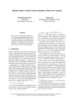
5.2 Discussion
The results clearly show that gains came from both
the switch from generative to discriminative train-
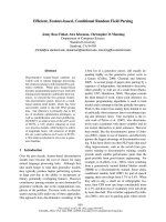
ing, and from the extensive use of features. In Fig-
ure 3 we show for an example from section 22 the
parse trees produced by our generative model and
our feature-based discriminative model, and the cor-
rect parse. The parse from the feature-based model
better exhibits the right branching tendencies of En-
glish. This is likely due to the heavy feature, which
encourages long constituents at the end of the sen-

tence. It is difficult for a standard PCFG to learn this
aspect of the English language, because the score it
assigns to a rule does not take its span into account.
4
The server does almost no computation.
964
Model P R F
1
Exact Avg CB 0 CB P R F
1
Exact Avg CB 0 CB
development set – length ≤ 15 test set – length ≤ 15
Taskar 2004 89.7 90.2 90.0 – – – 89.1 89.1 89.1 – – –
Turian 2007
– – – – – – 89.6 89.3 89.4 – – –
generative 86.9 85.8 86.4 46.2 0.34 81.2 87.6 85.8 86.7 49.2 0.33 81.9
discriminative 89.1 88.6 88.9 55.5 0.26 85.5 88.9 88.0 88.5 56.6 0.32 85.0
feature-based
90.4 89.3 89.9 59.5 0.24 88.3 91.1 90.2 90.6 61.3 0.24 86.8
relaxed 91.2 90.3 90.7 62.1 0.24 88.1 91.4 90.4 90.9 62.0 0.22 87.9
Table 3: Development and test set results, training and testing on sentences of length ≤ 15 from the Penn treebank.
Model
P R F
1
Exact Avg CB 0 CB P R F
1
Exact Avg CB 0 CB
test set – length ≤ 40 test set – all sentences
Petrov 2007 – – 88.8 – – – – – 88.3 – – –
generative 83.5 82.0 82.8 25.5 1.57 53.4 82.8 81.2 82.0 23.8 1.83 50.4

generative-all
83.6 82.1 82.8 25.2 1.56 53.3 – – – – – –
discriminative 85.1 84.5 84.8 29.7 1.41 55.8 84.2 83.7 83.9 27.8 1.67 52.8
feature-based
89.2 88.8 89.0 37.3 0.92 65.1 88.2 87.8 88.0 35.1 1.15 62.3
Table 4: Test set results, training on sentences of length ≤ 40 from the Penn treebank. The generative-all results were
trained on all sentences regardless of length
6 Comparison With Related Work
The most similar related work is (Johnson, 2001),
which did discriminative training of a generative
PCFG. The model was quite similar to ours, except
that it did not incorporate any features and it re-
quired the parameters (which were just scores for
rules) to be locally normalized, as with a genera-
tively trained model. Due to training time, they used
the ATIS treebank corpus , which is much smaller
than even WSJ15, with only 1,088 training sen-
tences, 294 testing sentences, and an average sen-
tence length of around 11. They found no signif-
icant difference in performance between their gen-
eratively and discriminatively trained parsers. There
are two probable reasons for this result. The training
set is very small, and it is a known fact that gener-
ative models tend to work better for small datasets
and discriminative models tend to work better for
larger datasets (Ng and Jordan, 2002). Additionally,
they made no use of features, one of the primary
benefits of discriminative learning.
Taskar et al. (2004) took a large margin approach
to discriminative learning, but achieved only small

gains. We suspect that this is in part due to the gram-
mar that they chose – the grammar of (Klein and
Manning, 2003), which was hand annotated with the
intent of optimizing performance of a PCFG. This
grammar is fairly sparse – for any particular state
there are, on average, only a few rules with that state
as a parent – so the learning algorithm may have suf-
fered because there were few options to discriminate
between. Starting with this grammar we found it dif-
ficult to achieve gains as well. Additionally, their
long training time (several months for WSJ15, ac-
cording to (Turian and Melamed, 2006)) made fea-
ture engineering difficult; they were unable to really
explore the space of possible features.
More recent is the work of (Turian and Melamed,
2006; Turian et al., 2007), which improved both the
training time and accuracy of (Taskar et al., 2004).
They define a simple linear model, use boosted de-
cision trees to select feature conjunctions, and a line
search to optimize the parameters. They use an
agenda parser, and define their atomic features, from
which the decision trees are constructed, over the en-
tire state being considered. While they make exten-
sive use of features, their setup is much more com-
plex than ours and takes substantially longer to train
– up to 5 days on WSJ15 – while achieving only
small gains over (Taskar et al., 2004).
The most recent similar research is (Petrov et al.,
2007). They also do discriminative parsing of length
40 sentences, but with a substantially different setup.

Following up on their previous work (Petrov et al.,
2006) on grammar splitting, they do discriminative
965
S
S
NP
PRP
He
VP
VBZ
adds
NP
DT
This
VP
VBZ
is
RB
n’t
NP
NP
CD
1987
VP
VBN
revisited
S
NP
PRP
He

VP
VBZ
adds
S
NP
DT
This
VP
VBZ
is
RB
n’t
NP
CD
1987
VP
VBN
revisited
S
NP
PRP
He
VP
VBZ
adds
S
NP
DT
This
VP

VBZ
is
RB
n’t
NP
NP
CD
1987
VP
VBN
revisited
(a) generative output (b) feature-based discriminative output (c) gold parse
Figure 3: Example output from our generative and feature-based discriminative models, along with the correct parse.
parsing with latent variables, which requires them
to optimize a non-convex function. Instead of us-
ing a stochastic optimization technique, they use L-
BFGS, but do coarse-to-fine pruning to approximate
their gradients and log likelihood. Because they
were focusing on grammar splitting they, like (John-
son, 2001), did not employ any features, and, like
(Taskar et al., 2004), they saw only small gains from
switching from generative to discriminative training.
7 Conclusions
We have presented a new, feature-rich, dynamic pro-
gramming based discriminative parser which is sim-
pler, more effective, and faster to train and test than
previous work, giving us new state-of-the-art per-
formance when training and testing on sentences of
length ≤ 15 and the first results for such a parser
trained and tested on sentences of length ≤ 40. We

also show that the use of SGD for training CRFs per-
forms as well as L-BFGS in a fraction of the time.
Other recent work on discriminative parsing has ne-
glected the use of features, despite their being one of
the main advantages of discriminative training meth-
ods. Looking at how other tasks, such as named
entity recognition and part-of-speech tagging, have
evolved over time, it is clear that greater gains are to
be gotten from developing better features than from
better models. We have provided just such a frame-
work for improving parsing performance.
Acknowledgments
Many thanks to Teg Grenager and Paul Heymann
for their advice (and their general awesomeness),
and to our anonymous reviewers for helpful com-
ments.
This paper is based on work funded in part by
the Defense Advanced Research Projects Agency
through IBM, by the Disruptive Technology Office
(DTO) Phase III Program for Advanced Question
Answering for Intelligence (AQUAINT) through
Broad Agency Announcement (BAA) N61339-06-
R-0034, and by a Scottish Enterprise Edinburgh-
Stanford Link grant (R37588), as part of the EASIE
project.
References
Eugene Charniak and Mark Johnson. 2005. Coarse-to-
fine n-best parsing and maxent discriminative rerank-
ing. In ACL 43, pages 173–180.
Alexander Clark. 2000. Inducing syntactic categories by

context distribution clustering. In Proc. of Conference
on Computational Natural Language Learning, pages
91–94, Lisbon, Portugal.
Trevor Cohn and Philip Blunsom. 2005. Semantic
role labelling with tree conditional random fields. In
CoNLL 2005.
Michael Collins. 2000. Discriminative reranking for nat-
ural language parsing. In ICML 17, pages 175–182.
Jay Earley. 1970. An efficient context-free parsing algo-
rithm. Communications of the ACM, 6(8):451–455.
James Henderson. 2004. Discriminative training of a
neural network statistical parser. In ACL 42, pages 96–
103.
Mark Johnson. 2001. Joint and conditional estimation of
tagging and parsing models. In Meeting of the Associ-
ation for Computational Linguistics, pages 314–321.
Florent Jousse, R´emi Gilleron, Isabelle Tellier, and Marc
Tommasi. 2006. Conditional Random Fields for XML
966
trees. In ECML Workshop on Mining and Learning in
Graphs.
Dan Klein and Christopher D. Manning. 2003. Accurate
unlexicalized parsing. In Proceedings of the Associa-
tion of Computational Linguistics (ACL).
John Lafferty, Andrew McCallum, and Fernando Pereira.
2001. Conditional Random Fields: Probabilistic mod-
els for segmenting and labeling sequence data. In
ICML 2001, pages 282–289. Morgan Kaufmann, San
Francisco, CA.
Dong C. Liu and Jorge Nocedal. 1989. On the limited

memory BFGS method for large scale optimization.
Math. Programming, 45(3, (Ser. B)):503–528.
Christopher D. Manning and Hinrich Sch¨utze. 1999.
Foundations of Statistical Natural Language Process-
ing. The MIT Press, Cambridge, Massachusetts.
Mitchell P. Marcus, Beatrice Santorini, and Mary Ann
Marcinkiewicz. 1993. Building a large annotated cor-
pus of English: The Penn Treebank. Computational
Linguistics, 19(2):313–330.
Andrew Ng and Michael Jordan. 2002. On discrimina-
tive vs. generative classifiers: A comparison of logistic
regression and naive bayes. In Advances in Neural In-
formation Processing Systems (NIPS).
Slav Petrov, Leon Barrett, Romain Thibaux, and Dan
Klein. 2006. Learning accurate, compact, and in-
terpretable tree annotation. In ACL 44/COLING 21,
pages 433–440.
Slav Petrov, Adam Pauls, and Dan Klein. 2007. Dis-
criminative log-linear grammars with latent variables.
In NIPS.
Adwait Ratnaparkhi. 1997. A linear observed time sta-
tistical parser based on maximum entropy models. In
EMNLP 2, pages 1–10.
Andreas Stolcke. 1995. An efficient probabilistic
context-free parsing algorithm that computes prefix
probabilities. Computational Linguistics, 21:165–
202.
Ben Taskar, Dan Klein, Michael Collins, Daphne Koller,
and Christopher D. Manning. 2004. Max-margin
parsing. In Proceedings of the Conference on Em-

pirical Methods in Natural Language Processing
(EMNLP).
Joseph Turian and I. Dan Melamed. 2006. Advances in
discriminative parsing. In ACL 44, pages 873–880.
Joseph Turian, Ben Wellington, and I. Dan Melamed.
2007. Scalable discriminative learning for natural lan-
guage parsing and translation. In Advances in Neural
Information Processing Systems 19, pages 1409–1416.
MIT Press.
S. V. N. Vishwanathan, Nichol N. Schraudolph, Mark W.
Schmidt, and Kevin P. Murphy. 2006. Accelerated
training of conditional random fields with stochastic
gradient methods. In ICML 23, pages 969–976.
967