Báo cáo khoa học: "Estimating Class Priors in Domain Adaptation for Word Sense Disambiguation" pdf
Bạn đang xem bản rút gọn của tài liệu. Xem và tải ngay bản đầy đủ của tài liệu tại đây (125.42 KB, 8 trang )
Proceedings of the 21st International Conference on Computational Linguistics and 44th Annual Meeting of the ACL, pages 89–96,
Sydney, July 2006.
c
2006 Association for Computational Linguistics
Estimating Class Priors in Domain Adaptation
for Word Sense Disambiguation
Yee Seng Chan and Hwee Tou Ng
Department of Computer Science
National University of Singapore
3 Science Drive 2, Singapore 117543
chanys,nght @comp.nus.edu.sg
Abstract
Instances of a word drawn from different
domains may have different sense priors
(the proportions of the different senses of
a word). This in turn affects the accuracy
of word sense disambiguation (WSD) sys-
tems trained and applied on different do-
mains. This paper presents a method to
estimate the sense priors of words drawn
from a new domain, and highlightstheim-
portance of using well calibrated probabil-
ities when performing these estimations.
By using well calibrated probabilities, we
are able to estimate the sense priors effec-
tively to achieve significant improvements
in WSD accuracy.
1 Introduction
Many words have multiple meanings, and the pro-
cess of identifying the correct meaning, or sense
of a word in context, is known as word sense
disambiguation (WSD). Among the various ap-
proaches to WSD, corpus-based supervised ma-
chine learning methods have been the most suc-
cessful to date. With this approach, one would
need to obtain a corpus in which each ambiguous
word has been manually annotated with the correct
sense, to serve as training data.
However, supervised WSD systems faced an
important issue of domain dependence when using
such a corpus-based approach. To investigate this,
Escudero et al. (2000) conducted experiments
using the DSO corpus, which contains sentences
drawn from two different corpora, namely Brown
Corpus (BC) and Wall Street Journal (WSJ). They
found that training a WSD system on one part (BC
or WSJ) of the DSO corpus and applying it to the
other part can result in an accuracy drop of 12%
to 19%. One reason for this is the difference in
sense priors (i.e., the proportions of the different
senses of a word) between BC and WSJ. For in-
stance, the noun interest has these 6 senses in the
DSO corpus: sense 1, 2, 3, 4, 5, and 8. In the BC
part of the DSO corpus, these senses occur with
the proportions: 34%, 9%, 16%, 14%, 12%, and
15%. However, in the WSJ part of the DSO cor-
pus, the proportions are different: 13%, 4%, 3%,
56%, 22%, and 2%. When the authors assumed
they knew the sense priors of each word in BC and
WSJ, and adjusted these two datasets such that the
proportions of the different senses of each word
were the same between BC and WSJ, accuracy im-
proved by 9%. In another work, Agirre and Mar-
tinez (2004) trained a WSD system on data which
was automatically gathered from the Internet. The
authors reported a 14% improvement in accuracy
if they have an accurate estimate of the sense pri-
ors in the evaluation data and sampled their train-
ing data according to these sense priors. The work
of these researchers showed that when the domain
of the training data differs from the domain of the
data on which the system is applied, there will be
a decrease in WSD accuracy.
To build WSD systems that are portable across
different domains, estimation of the sense priors
(i.e., determining the proportions of the differ-
ent senses of a word) occurring in a text corpus
drawn from a domain is important. McCarthy et
al. (2004) provideda partial solutionby describing
a method to predict the predominant sense, or the
most frequent sense, of a word in a corpus. Using
the noun interest as an example, their method will
try to predict that sense 1 is the predominant sense
in the BC part of the DSO corpus, while sense 4
is the predominant sense in the WSJ part of the
89
corpus.
In our recent work (Chan and Ng, 2005b), we
directly addressed the problem by applying ma-
chine learning methods to automatically estimate
the sense priors in the target domain. For instance,
given the noun interest and the WSJ part of the
DSO corpus, we attempt to estimate the propor-
tion of each sense of interest occurring in WSJ and
showed that these estimates help to improve WSD
accuracy. In our work, we used naive Bayes as
the training algorithm to provide posterior proba-
bilities, or class membership estimates, for the in-
stances in the target domain. These probabilities
were then used by the machine learning methods
to estimate the sense priors of each word in the
target domain.
However, it is known that the posterior proba-
bilitiesassignedby naive Bayes are not reliable, or
not well calibrated (Domingos and Pazzani, 1996).
These probabilities are typically too extreme, of-
ten being very near 0 or 1. Since these probabil-
ities are used in estimating the sense priors, it is
important that they are well calibrated.
In this paper, we explore the estimation of sense
priors by first calibrating the probabilities from
naive Bayes. We also propose using probabilities
from another algorithm (logistic regression, which
already gives well calibrated probabilities) to esti-
mate the sense priors. We show that by using well
calibrated probabilities, we can estimate the sense
priors more effectively. Using these estimates im-
proves WSD accuracy and we achieve results that
are significantly better than using our earlier ap-
proach described in (Chan and Ng, 2005b).
In the following section, we describe the algo-
rithm to estimate the sense priors. Then, we de-
scribe the notion of being well calibrated and dis-
cuss why using well calibrated probabilities helps
in estimating the sense priors. Next, we describe
an algorithm to calibrate the probability estimates
from naive Bayes. Then, we discuss the corpora
and the set of words we use for our experiments
before presenting our experimental results. Next,
we propose using the well calibrated probabilities
of logistic regression to estimate the sense priors,
and perform significance tests to compare our var-
ious results before concluding.
2 Estimation of Priors
To estimate the sense priors, or a priori proba-
bilities of the different senses in a new dataset,
we used a confusion matrix algorithm (Vucetic
and Obradovic, 2001) and an EM based algorithm
(Saerens et al., 2002) in (Chan and Ng, 2005b).
Our results in (Chan and Ng, 2005b) indicate that
the EM based algorithm is effective in estimat-
ing the sense priors and achieves greater improve-
ments in WSD accuracy compared to the confu-
sion matrix algorithm. Hence, to estimate the
sense priors in our current work, we use the EM
based algorithm, which we describe in this sec-
tion.
2.1 EM Based Algorithm
Most of this section is based on (Saerens et al.,
2002). Assume we have a set of labeled data D
with n classes and a set of N independent instances
from a new data set. The likelihood
of these N instances can be defined as:
(1)
Assuming the within-class densities ,
i.e., the probabilities of observing given the
class , do not change from the training set D
to the new data set, we can define:
. To determine the a priori probability
estimates of the new data set that will max-
imize the likelihood of (1) with respect to ,
we can apply the iterative procedure of the EM al-
gorithm. In effect, through maximizing the likeli-
hood of (1), we obtain the a priori probability es-
timates as a by-product.
Let us now define some notations. When we
apply a classifier trained on D on an instance
drawn from the new data set D , we get
, which we define as the probability of
instance being classified as class by the clas-
sifier trained on D . Further, let us define
as the a priori probabilities of class in D . This
can be estimated by the class frequency of in
D . We also define and as es-
timates of the new a priori and a posteriori proba-
bilities at step s of the iterative EM procedure. As-
suming we initialize
, then for
each instance in D and each class , the EM
90
algorithm provides the following iterative steps:
(2)
(3)
where Equation (2) represents the expectation E-
step, Equation (3) represents the maximization M-
step, and N represents the number of instances in
D . Note that the probabilities and
in Equation (2) will stay the same through-
out the iterations for each particular instance
and class . The new a posteriori probabilities
at step s in Equation (2) are simply the
a posteriori probabilities in the conditions of the
labeled data, , weighted by the ratio of
the new priors to the old priors .
The denominator in Equation (2) is simply a nor-
malizing factor.
The a posteriori and a priori proba-
bilities are re-estimated sequentially dur-
ing each iteration s for each new instance and
each class , until the convergence of the esti-
mated probabilities . This iterative proce-
dure will increase the likelihoodof (1) at each step.
2.2 Using A Priori Estimates
If a classifier estimates posterior class probabili-
ties when presented witha newinstance
from D , it can be directly adjusted according
to estimated a priori probabilities on D :
(4)
where denotes the a priori probability of
class from D and denotes the
adjusted predictions.
3 Calibration of Probabilities
In our eariler work (Chan and Ng, 2005b), the
posterior probabilities assigned by a naive Bayes
classifier are used by the EM procedure described
in the previous section to estimate the sense pri-
ors in a new dataset. However, it is known
that the posterior probabilities assigned by naive
Bayes are not well calibrated (Domingos and Paz-
zani, 1996).
It is important to use an algorithm which gives
well calibrated probabilities, if we are to use the
probabilities in estimating the sense priors. In
this section, we will first describe the notion of
being well calibrated before discussing why hav-
ing well calibrated probabilities helps in estimat-
ing the sense priors. Finally, we will introduce
a method used to calibrate the probabilities from
naive Bayes.
3.1 Well Calibrated Probabilities
Assume for each instance , a classifier out-
puts a probability S between 0 and 1, of
belonging to class . The classifier is well-
calibrated if the empirical class membership prob-
ability S converges to the proba-
bility value S as the number of examples
classified goes to infinity (Zadrozny and Elkan,
2002). Intuitively, if we consider all the instances
to which the classifier assigns a probabilityS
of say 0.6, then 60% of these instances should be
members of class .
3.2 Being Well Calibrated Helps Estimation
To see why using an algorithm which gives well
calibrated probabilities helps in estimating the
sense priors, let us rewrite Equation (3), the M-
step of the EM procedure, as the following:
(5)
where S = denotes the set of poste-
rior probability values for class , and S
denotes the posterior probability of class as-
signed by the classifier for instance .
Based on , we can imagine that we
have bins, where each bin is associated with a
specific value. Now, distribute all the instances
in the new dataset D into the bins according
to their posterior probabilities . Let B , for
, denote the set of instances in bin .
Note that B B B = .
Now, let denote the proportion of instances with
true class label in B . Given a well calibrated
algorithm, by definition and Equation (5)
can be rewritten as:
B B
B B
(6)
91
Input: training set sorted in ascending order of
Initialize
While k such that , where
and
Set
Replace with m
Figure 1: PAV algorithm.
where denotes the number of instances in D
with true class label . Therefore, re-
flects the proportion of instances in D with true
class label . Hence, using an algorithm which
gives well calibrated probabilities helps in the es-
timation of sense priors.
3.3 Isotonic Regression
Zadrozny and Elkan (2002) successfully used a
method based on isotonic regression (Robertson
et al., 1988) to calibrate the probability estimates
from naive Bayes. To compute the isotonic regres-
sion, they used the pair-adjacent violators (PAV)
(Ayer et al., 1955) algorithm, which we show in
Figure 1. Briefly, what PAV does is to initially
view each data value as a level set. While there
are two adjacent sets that are out of order (i.e., the
left level set is above the right one) then the sets
are combined and the mean of the data values be-
comes the value of the new level set.
PAV works on binary class problems. In
a binary class problem, we have a positive
class and a negative class. Now, let
, where represent
N examples and is the probability of belong-
ing to the positive class, as predicted by a classi-
fier. Further, let represent the true label of .
For a binary class problem, we let if
is a positive example and if is a neg-
ative example. The PAV algorithm takes in a set
of , sorted in ascending order of and re-
turns a series of increasing step-values,where each
step-value (denoted by m in Figure 1) is associ-
ated with a lowestboundary value and a highest
boundary value . We performed 10-fold cross-
validation on the training data to assign values to
. We then applied the PAV algorithm to obtain
values for . To obtain the calibrated probability
estimate for a test instance , we find the bound-
ary values and where S and
assign as the calibrated probability estimate.
To apply PAV on a multiclass problem, we first
reduce the problem into a number of binary class
problems. For reducing a multiclass problem into
a set of binary class problems, experiments in
(Zadrozny and Elkan, 2002) suggest that the one-
against-all approach works well. In one-against-
all, a separate classifier is trained for each class ,
where examples belonging to class are treated
as positive examples and all other examples are
treated as negative examples. A separate classifier
is then learnt for each binary class problem and the
probability estimates from each classifier are cali-
brated. Finally, the calibrated binary-class proba-
bility estimates are combined to obtain multiclass
probabilities, computed by a simple normalization
of the calibrated estimates from each binary clas-
sifier, as suggested by Zadrozny and Elkan (2002).
4 Selection of Dataset
In this section, we discuss the motivations in
choosing the particular corpora and the set of
words used in our experiments.
4.1 DSO Corpus
The DSO corpus (Ng and Lee, 1996) contains
192,800 annotated examples for 121 nouns and 70
verbs, drawn from BC and WSJ. BC was built as a
balanced corpus and contains texts in various cate-
gories such as religion, fiction, etc. In contrast, the
focus of the WSJ corpus is on financial and busi-
ness news. Escudero et al. (2000) exploited the
difference in coverage between these two corpora
to separate the DSO corpus into its BC and WSJ
parts for investigating the domain dependence of
several WSD algorithms. Following their setup,
we also use the DSO corpus in our experiments.
The widely used SEMCOR (SC) corpus (Miller
et al., 1994) is one of the few currently avail-
able manually sense-annotated corpora for WSD.
SEMCOR is a subset of BC. Since BC is a bal-
anced corpus, and training a classifier on a general
corpus before applying it to a more specific corpus
is a natural scenario, we will use examples from
BC as training data, and examples from WSJ as
evaluation data, or the target dataset.
4.2 Parallel Texts
Scalability is a problem faced by current super-
vised WSD systems, as they usually rely on man-
ually annotated data for training. To tackle this
problem, in one of our recent work (Ng et al.,
2003), we had gathered training data from paral-
lel texts and obtained encouraging results in our
92
evaluation on the nouns of SENSEVAL-2 English
lexical sample task (Kilgarriff, 2001). In another
recent evaluation on the nouns of SENSEVAL-
2 English all-words task (Chan and Ng, 2005a),
promising results were also achieved using exam-
ples gathered from parallel texts. Due to the po-
tential of parallel texts in addressing the issue of
scalability, we also drew training data for our ear-
lier sense priors estimation experiments (Chan and
Ng, 2005b) from parallel texts. In addition, our
parallel texts training data represents a natural do-
main difference with the test data of SENSEVAL-
2 English lexical sample task, of which 91% is
drawn from the British National Corpus (BNC).
As part of our experiments, we followed the ex-
perimental setup of our earlier work (Chan and
Ng, 2005b), using the same 6 English-Chinese
parallel corpora (Hong Kong Hansards, Hong
Kong News, Hong Kong Laws, Sinorama, Xinhua
News, and English translation of Chinese Tree-
bank), available from LinguisticData Consortium.
To gather training examples from these parallel
texts, we used the approach we described in (Ng
et al., 2003) and (Chan and Ng, 2005b). We
then evaluated our estimation of sense priors on
the nouns of SENSEVAL-2 English lexical sam-
ple task, similar to the evaluation we conducted
in (Chan and Ng, 2005b). Since the test data for
the nouns of SENSEVAL-3Englishlexical sample
task (Mihalcea et al., 2004) were also drawn from
BNC and represented a difference in domain from
the parallel texts we used, we also expanded our
evaluation to these SENSEVAL-3 nouns.
4.3 Choice of Words
Research by (McCarthy et al., 2004) highlighted
that the sense priors of a word in a corpus depend
on the domain from which the corpus is drawn.
A change of predominant sense is often indicative
of a change in domain, as different corpora drawn
from different domains usually give different pre-
dominant senses. For example, the predominant
sense of the noun interest in the BC part of the
DSO corpus has the meaning “a sense of concern
with and curiosity about someone or something”.
In the WSJ part of the DSO corpus, the noun in-
terest has a different predominant sense with the
meaning “a fixed charge for borrowing money”,
reflecting the business and finance focus of the
WSJ corpus.
Estimation of sense priors is important when
there is a significant change in sense priors be-
tween the training and target dataset, such as when
there is a change in domain between the datasets.
Hence, in our experiments involving the DSO cor-
pus, we focused on the set of nouns and verbs
which had different predominant senses between
the BC and WSJ parts of the corpus. This gave
us a set of 37 nouns and 28 verbs. For experi-
ments involving the nouns of SENSEVAL-2 and
SENSEVAL-3 English lexical sample task, we
used the approach we described in (Chan and Ng,
2005b) of sampling training examples from the
parallel texts using the natural (empirical) distri-
bution of examples in the parallel texts. Then, we
focused on the set of nouns having different pre-
dominant senses between the examples gathered
from parallel texts and the evaluation data for the
two SENSEVAL tasks. This gave a set of 6 nouns
for SENSEVAL-2 and 9 nouns for SENSEVAL-
3. For each noun, we gathered a maximum of 500
parallel text examples as training data, similar to
what we had done in (Chan and Ng, 2005b).
5 Experimental Results
Similar to our previous work (Chan and Ng,
2005b), we used the supervised WSD approach
described in (Lee and Ng, 2002) for our exper-
iments, using the naive Bayes algorithm as our
classifier. Knowledge sources used include parts-
of-speech, surrounding words, and local colloca-
tions. This approach achieves state-of-the-art ac-
curacy. All accuracies reported in our experiments
are micro-averages over all test examples.
In (Chan and Ng, 2005b), we used a multiclass
naive Bayes classifier (denoted by NB) for each
word. Followingthis approach, we noted the WSD
accuracies achieved withoutany adjustment, in the
column L under NB in Table 1. The predictions
of these naive Bayes classifiers are then
used in Equation (2) and (3) to estimate the sense
priors , before being adjusted by these esti-
mated sense priors based on Equation (4). The re-
sulting WSD accuracies after adjustment are listed
in the column EM in Table 1, representing the
WSD accuracies achievable by following the ap-
proach we described in (Chan and Ng, 2005b).
Next, we used the one-against-all approach to
reduce each multiclass problem into a set of binary
class problems. We trained a naive Bayes classifier
for each binary problem and calibrated the prob-
abilities from these binary classifiers. The WSD
93
Classifier NB NBcal
Method L EM EM L EM EM
DSO nouns 44.5 46.1 46.6 45.8 47.0 51.1
DSO verbs 46.7 48.3 48.7 46.9 49.5 50.8
SE2 nouns 61.7 62.4 63.0 62.3 63.2 63.5
SE3 nouns 53.9 54.9 55.7 55.4 58.8 58.4
Table 1: Micro-averaged WSD accuracies using the various methods. The different naive Bayes classifiers are: multiclass
naive Bayes (NB) and naive Bayes with calibrated probabilities (NBcal).
Dataset True L EM L EM L
DSO nouns 11.6 1.2 (10.3%) 5.3 (45.7%)
DSO verbs 10.3 2.6 (25.2%) 3.9 (37.9%)
SE2 nouns 3.0 0.9 (30.0%) 1.2 (40.0%)
SE3 nouns 3.7 3.4 (91.9%) 3.0 (81.1%)
Table 2: Relative accuracy improvement based on cali-
brated probabilities.
accuracies of these calibrated naive Bayes classi-
fiers (denoted by NBcal) are given in the column L
under NBcal.
1
The predictions of these classifiers
are then used to estimate the sense priors
,
before being adjusted by these estimates based on
Equation (4). The resulting WSD accuracies after
adjustment are listed in column EM in Table
1.
The results show that calibrating the proba-
bilities improves WSD accuracy. In particular,
EM achieves the highest accuracy among the
methods described so far. To provide a basis for
comparison, we also adjusted the calibrated prob-
abilities by the true sense priors of the test
data. The increase in WSD accuracy thus ob-
tained is given in the column True L in Table
2. Note that this represents the maximum possi-
ble increase in accuracy achievable provided we
know these true sense priors . In the col-
umn EM in Table 2, we list the increase
in WSD accuracy when adjusted by the sense pri-
ors which were automatically estimated us-
ing the EM procedure. The relative improvements
obtained with using (compared against us-
ing ) are given as percentages in brackets.
As an example, according to Table 1 for the DSO
verbs, EM gives an improvement of 49.5%
46.9% = 2.6% in WSD accuracy, and the rela-
tive improvement compared tousingthetruesense
priors is 2.6/10.3 = 25.2%, as shown in Table 2.
Dataset EM EM EM
DSO nouns 0.621 0.586 0.293
DSO verbs 0.651 0.602 0.307
SE2 nouns 0.371 0.307 0.214
SE3 nouns 0.693 0.632 0.408
Table 3: KL divergence between the true and estimated
sense distributions.
6 Discussion
The experimental results show that the sense
priors estimated using the calibrated probabilities
of naive Bayes are effective in increasing the WSD
accuracy. However, using a learning algorithm
which already gives well calibrated posterior prob-
abilities may be more effective in estimating the
sense priors. One possible algorithm is logis-
tic regression, which directly optimizes for get-
ting approximations of the posterior probabilities.
Hence, its probability estimates are already well
calibrated (Zhang and Yang, 2004; Niculescu-
Mizil and Caruana, 2005).
In the rest of this section, we first conduct ex-
periments to estimate sense priors using the pre-
dictions of logistic regression. Then, we perform
significance tests to compare the various methods.
6.1 Using Logistic Regression
We trained logistic regression classifiers and eval-
uated them on the 4 datasets. However, the WSD
accuracies of these unadjusted logistic regression
classifiers are on average about 4% lower than
those of the unadjusted naive Bayes classifiers.
One possible reason is that being a discriminative
learner, logistic regression requires more train-
ing examples for its performance to catch up to,
and possibly overtake the generative naive Bayes
learner (Ng and Jordan, 2001).
Although the accuracy of logistic regression as
a basic classifier is lower than that of naive Bayes,
its predictions may still be suitable for estimating
1
Though not shown, we also calculated the accuracies of
these binary classifiers without calibration, and found them
to be similar to the accuracies of the multiclass naive Bayes
shown in the column L under NB in Table 1.
94
Method comparison DSO nouns DSO verbs SE2 nouns SE3 nouns
NB-EM vs. NB-EM
NBcal-EM vs. NB-EM
NBcal-EM vs. NB-EM
NBcal-EM vs. NB-EM
NBcal-EM vs. NB-EM
NBcal-EM vs. NBcal-EM
Table 4: Paired t-tests between the various methods for the 4 datasets.
sense priors. To gauge how well the sense pri-
ors are estimated, we measure the KL divergence
between the true sense priors and the sense pri-
ors estimated by using the predictions of (uncal-
ibrated) multiclass naive Bayes, calibrated naive
Bayes, and logistic regression. These results are
shown in Table 3 and the column EM shows
that using the predictions of logistic regression to
estimate sense priors consistently gives the lowest
KL divergence.
Results of the KL divergence test motivate us to
use sense priors estimated by logistic regression
on the predictions of the naive Bayes classifiers.
To elaborate, we first use the probability estimates
of logistic regression in Equations (2)
and (3) to estimate the sense priors . These
estimates and the predictions of
the calibrated naive Bayes classifier are then used
in Equation (4) to obtain the adjusted predictions.
The resulting WSD accuracy is shown in the col-
umn EM under NBcal in Table 1. Corre-
sponding results when the predictions
of the multiclass naive Bayes is used in Equation
(4), are given in the column EM under NB.
The relative improvements against using the true
sense priors, based on the calibrated probabilities,
are given in the column EM L in Table 2.
The results show that the sense priors provided by
logistic regression are in general effective in fur-
ther improving the results. In the case of DSO
nouns, this improvement is especially significant.
6.2 Significance Test
Paired t-tests were conducted to see if one method
is significantly better than another. The t statistic
of the difference between each test instance pair is
computed, giving rise to a p value. The results of
significance tests for the various methods on the 4
datasets are given in Table 4, where the symbols
“ ”, “ ”, and “ ” correspond to p-value 0.05,
(0.01, 0.05], and 0.01 respectively.
The methods in Table 4 are represented in the
form a1-a2, where a1 denotes adjusting the pre-
dictions of which classifier, and a2 denotes how
the sense priors are estimated. As an example,
NBcal-EM specifies that the sense priors es-
timated by logistic regression is used to adjust the
predictions of the calibrated naive Bayes classifier,
and corresponds to accuracies in column EM
under NBcal in Table 1. Based on the signifi-
cance tests, the adjusted accuracies of EM and
EM in Table 1 are significantly better than
their respective unadjusted L accuracies, indicat-
ing that estimating the sense priors of a new do-
main via the EM approach presented in this paper
significantly improves WSD accuracy compared
to just using the sense priors from the old domain.
NB-EM
represents our earlier approach in
(Chan and Ng, 2005b). The significance tests
show that our current approach of using calibrated
naive Bayes probabilities to estimate sense priors,
and then adjusting the calibrated probabilities by
these estimates (NBcal-EM ) performs sig-
nificantly better than NB-EM (refer to row 2
of Table 4). For DSO nouns, though the results
are similar, the p value is a relatively low 0.06.
Using sense priors estimated by logistic regres-
sion further improves performance. For example,
row 1 of Table 4 shows that adjusting the pre-
dictions of multiclass naive Bayes classifiers by
sense priors estimated by logistic regression (NB-
EM ) performs significantly better than using
sense priors estimated by multiclass naive Bayes
(NB-EM ). Finally, using sense priors esti-
mated by logistic regression to adjust the predic-
tions of calibrated naive Bayes (NBcal-EM )
in general performs significantly better than most
other methods, achieving the best overall perfor-
mance.
In addition, we implemented the unsupervised
method of (McCarthy et al., 2004), which calcu-
lates a prevalence score for each sense of a word
to predict the predominant sense. As in our earlier
work (Chan and Ng, 2005b), we normalized the
prevalence score of each sense to obtain estimated
sense priors for each word, which we then used
95
to adjust the predictions of our naive Bayes classi-
fiers. We found that the WSD accuracies obtained
with the method of (McCarthy et al., 2004) are
on average 1.9% lower than our NBcal-EM
method, and the difference is statistically signifi-
cant.
7 Conclusion
Differences in sense priors between training and
target domain datasets will result in a loss of WSD
accuracy. In this paper, we show that using well
calibrated probabilities to estimate sense priors is
important. By calibrating the probabilities of the
naive Bayes algorithm, and using the probabilities
given by logistic regression (which is already well
calibrated), we achieved significant improvements
in WSD accuracy over previous approaches.
References
Eneko Agirre and David Martinez. 2004. Unsuper-
vised WSD based on automatically retrieved exam-
ples: The importance of bias. In Proc. ofEMNLP04.
Miriam Ayer, H. D. Brunk, G. M. Ewing, W. T. Reid,
and Edward Silverman. 1955. An empirical distri-
bution function for sampling with incomplete infor-
mation. Annals of Mathematical Statistics, 26(4).
Yee Seng Chan and Hwee Tou Ng. 2005a. Scaling
up word sense disambiguation via parallel texts. In
Proc. of AAAI05.
Yee Seng Chan and Hwee Tou Ng. 2005b. Word
sense disambiguation with distribution estimation.
In Proc. of IJCAI05.
Pedro Domingos and Michael Pazzani. 1996. Beyond
independence: Conditions for the optimality of the
simple Bayesian classifier. In Proc. of ICML-1996.
Gerard Escudero, Lluis Marquez, and German Rigau.
2000. An empirical study of the domain dependence
of supervised word sense disambiguation systems.
In Proc. of EMNLP/VLC00.
Adam Kilgarriff. 2001. English lexical sample task
description. In Proc. of SENSEVAL-2.
Yoong Keok Lee and Hwee Tou Ng. 2002. An empir-
ical evaluation of knowledge sources and learning
algorithms for word sense disambiguation. In Proc.
of EMNLP02.
Diana McCarthy, Rob Koeling, Julie Weeds, and John
Carroll. 2004. Finding predominant word senses in
untagged text. In Proc. of ACL04.
Rada Mihalcea, Timothy Chklovski, and Adam Kilgar-
riff. 2004. The senseval-3 english lexical sample
task. In Proc. of SENSEVAL-3.
George A. Miller, Martin Chodorow, Shari Landes,
Claudia Leacock, and Robert G. Thomas. 1994.
Using a semantic concordance for sense identifica-
tion. In Proc. of ARPA Human Language Technol-
ogy Workshop.
Andrew Y. Ng and Michael I. Jordan. 2001. On dis-
criminative vs. generative classifiers: A comparison
of logistic regression and naive Bayes. In Proc. of
NIPS14.
Hwee Tou Ng and Hian Beng Lee. 1996. Integrating
multiple knowledge sources to disambiguate word
sense: An exemplar-based approach. In Proc. of
ACL96.
Hwee Tou Ng, Bin Wang, and Yee Seng Chan. 2003.
Exploiting parallel texts for word sense disambigua-
tion: An empirical study. In Proc. of ACL03.
Alexandru Niculescu-Mizil and Rich Caruana. 2005.
Predicting good probabilities with supervised learn-
ing. In Proc. of ICML05.
Tim Robertson, F. T. Wright, and R. L. Dykstra. 1988.
Chapter 1. Isotonic Regression. In Order Restricted
Statistical Inference. John Wiley & Sons.
Marco Saerens, Patrice Latinne, and Christine De-
caestecker. 2002. Adjusting the outputs of a clas-
sifier to new a priori probabilities: A simple proce-
dure. Neural Computation,14(1).
Slobodan Vucetic and Zoran Obradovic. 2001. Clas-
sification on data with biased class distribution. In
Proc. of ECML01.
Bianca Zadrozny and Charles Elkan. 2002. Trans-
forming classifier scores into accurate multiclass
probability estimates. In Proc. of KDD02.
Jian Zhang and Yiming Yang. 2004. Probabilistic
score estimation with piecewise logistic regression.
In Proc. of ICML04.
96