Microsoft excel advanced functions and formulas
Bạn đang xem bản rút gọn của tài liệu. Xem và tải ngay bản đầy đủ của tài liệu tại đây (3.76 MB, 93 trang )
Excel Advanced
Functions and Formulas
Ahmed Sheikh, M.Sc. (USA)
TABLE OF CONTENTS
Unit 1: Building complex formulas .....................................................................................................4
Using nested IF statements....................................................................................................................... 4
Creating compound logical tests using AND, OR, NOT functions with IF statements .............................. 5
Comparing a nested IF formula with VLOOKUP .................................................................................... 7
Using the NOT function......................................................................................................................... 7
Nesting VLOOKUP functions ..................................................................................................................... 8
Using VLOOKUP with the COLUMN function ........................................................................................ 8
Source table structure information using CHOOSE function .................................................................. 10
Compare the CHOOSE function with Nested IF with INDEX.................................................................... 11
Using the MATCH function to locate data position ................................................................................ 14
Match Types ........................................................................................................................................ 14
Use the INDEX function for retrieving information by location .............................................................. 16
The INDEX Array form ......................................................................................................................... 16
Using a nested formula containing INDEX, MATCH and MATCH (two-way lookup) .............................. 18
Unit 2: Using Advanced Functions..................................................................................................... 19
Use COUNTIFS and SUMIFS .................................................................................................................... 19
Using COUNTIF with OR logic .............................................................................................................. 21
Creating Tabulated data using SUMIFS .................................................................................................. 21
Creating Tabulated data with a Data Table ........................................................................................ 23
Using Statistical functions MEDIAN, RANK, MODE, LARGE, SMALL ....................................................... 25
RANK and RANK.AVG Function ........................................................................................................... 25
MEDIAN function ................................................................................................................................ 26
The MODE function............................................................................................................................. 27
The LARGE and SMALL functions. ....................................................................................................... 27
Use Maths functions: Round and related functions, the Mod function .................................................. 29
ROUND and related functions............................................................................................................. 29
MOD function ..................................................................................................................................... 32
Use the AGGREGATE function to sum data in ranges with errors .......................................................... 36
Use a variety of Financial functions such as PMT, FV, IRR ...................................................................... 39
PMT ..................................................................................................................................................... 39
FV ........................................................................................................................................................ 40
IRR ....................................................................................................................................................... 42
Unit 3: Date & Text Functions ........................................................................................................... 44
Calculating Dates and Times using TODAY, NETWORKDAYS, WORKDAY and DATEDIF ......................... 44
TODAY ................................................................................................................................................. 44
NETWORKDAYS ................................................................................................................................... 44
WORKDAY ........................................................................................................................................... 45
DATEDIF .............................................................................................................................................. 46
Creating Timesheets ........................................................................................................................... 50
Use Text Functions .................................................................................................................................. 51
LEFT ..................................................................................................................................................... 51
FIND..................................................................................................................................................... 53
SEARCH................................................................................................................................................ 53
PROPER ............................................................................................................................................... 54
UPPER and LOWER .............................................................................................................................. 55
LEN ...................................................................................................................................................... 55
TYPE..................................................................................................................................................... 56
TRIM .................................................................................................................................................... 57
CONCATENATE .................................................................................................................................... 58
Unit 4: Array formulas ..................................................................................................................... 59
Understanding Array Formulas............................................................................................................... 59
A multicell array formula .................................................................................................................... 60
Multi-cell array block formula............................................................................................................. 62
A single-cell array formula .................................................................................................................. 64
Creating an array constant ..................................................................................................................... 65
Array constant elements ..................................................................................................................... 65
Understanding the Dimensions of an Array............................................................................................ 66
One-dimensional horizontal arrays..................................................................................................... 66
One-dimensional vertical arrays ......................................................................................................... 66
Two-dimensional arrays ...................................................................................................................... 67
Naming Array Constants ..................................................................................................................... 68
Using TRANPOSE to insert a horizontal array into a vertical range of cells ........................................ 69
Using INDEX to access individual elements from an array ................................................................. 69
Working with Array Formulas ................................................................................................................. 69
Entering an array formula ................................................................................................................... 69
Selecting an array formula range ........................................................................................................ 69
Editing an array formula ..................................................................................................................... 69
Unit 5: Auditing Formulas................................................................................................................. 71
Trace Formula Precedents, Dependents and Errors ............................................................................... 71
Correcting Errors in Formulas ................................................................................................................. 73
Combine IF with VLOOKUP to suppress error messages......................................................................... 75
The IS Information Function.................................................................................................................... 77
Error Checking Functions; ISERR, ISERROR and IFERROR ........................................................................ 78
ISERR Function .................................................................................................................................... 78
ISERROR Function ............................................................................................................................... 79
IFERROR............................................................................................................................................... 79
IFERROR as an Array Formula ............................................................................................................. 80
Function syntax notes ...................................................................................................................... 81
IF.......................................................................................................................................................... 81
CHOOSE ............................................................................................................................................... 81
INDEX .................................................................................................................................................. 81
MATCH ................................................................................................................................................ 81
INDEX .................................................................................................................................................. 82
MATCH ................................................................................................................................................ 82
RANK ................................................................................................................................................... 83
RANK.AVG ........................................................................................................................................... 83
MEDIAN ............................................................................................................................................... 84
MODE .................................................................................................................................................. 84
ROUND ................................................................................................................................................ 84
ROUNDUP ........................................................................................................................................... 84
ROUNDDOWN ..................................................................................................................................... 85
PMT ..................................................................................................................................................... 85
FV ........................................................................................................................................................ 85
TODAY ................................................................................................................................................. 86
NETWORKDAYS ................................................................................................................................... 86
DATEDIF .............................................................................................................................................. 86
WORKDAY ........................................................................................................................................... 86
LEFT ..................................................................................................................................................... 86
RIGHT .................................................................................................................................................. 87
SEARCH................................................................................................................................................ 87
FIND..................................................................................................................................................... 87
LEN ...................................................................................................................................................... 87
MID...................................................................................................................................................... 87
ISERR ................................................................................................................................................... 87
ISERROR............................................................................................................................................... 88
IFERROR............................................................................................................................................... 88
Excel Advanced Part 2 Functions ...................................................................................................... 89
Unit 1: Building complex formulas
In this unit, you will learn how to:
Work with nesting functions
Compare results between using a formula with nested IF vs. a VLOOKUP
Use the VLOOKUP with the COLUMN function
Source table structure information using CHOOSE function
Use INDEX and MATCH to search for information
Formulas and worksheet functions are essential to manipulating data and obtaining useful information
from your Excel workbooks. This section includes formulas containing functions such as IF, AND, OR,
NOT, CHOOSE, VLOOKUP, COLUMN, INDEX and MATCH and to make it more challenging the examples
that will be used include combinations of these functions in the same formula.
Using nested IF statements
In Excel the 'IF' function is commonly used as it provides solutions for many complex and varying
situations in Excel. Let's begin with a formula containing multiple IF functions, also known as a nested IF
formula. It is necessary to understand the syntax of this function which is as follows:
IF(Logical Test, Value if True, IF(Logical Test, Value if True, IF(Logical Test, Value if True, Value if False)))
In the above example there are three logical tests which produce a value if true followed by a final result
if none of the IF statements are true. The following is an example showing grading comments based on
score results.
=IF(F2>=90,"Excellent", IF(F2>=70,"Very Good", IF(F2>=50,"Fair","Poor")))
To examine the formulas in more detail take a look at the following screenshot showing the breakdown
of the nested IF formula which produces the required results.
Creating compound logical tests using AND, OR, NOT functions with IF
statements
Using an IF function by itself in a formula works when there are no special conditions to be added. When
the results are based on conditions then you have to nest the IF function with either the AND function or
with the OR function. The AND function can hold up to 255 logical tests, however, to arrive at a result
which is TRUE all the logical tests must be true. This makes the AND function quite restrictive in its use.
On the other hand the OR function, which can also hold up to 255 logical tests, requires that only one of
its logical tests be true in order to arrive at a result which is TRUE.
In the following screenshot the Excel spreadsheet represents sales data and we will be using the IF
function together with AND, NOT and VLOOKUP to work out bonus calculations.
To pay a 2% bonus for sales greater than £20000 we would use a formula with a simple IF function that
would be as follows: -
=IF(F2>20000,0.02*F2,0)
But what if we decided that the bonus would only be paid if the GP% is greater than 50% in addition to
the first condition that sales must be greater than £20000? We could then use two IF functions one to
deal with the first logical test and then the second to deal with the new logical test. The formula to
produce the desired result would look like this: -
=IF(F2>20000,IF(I2>0.5,0.02*F2,0),0)
The exact same result can be achieved by using the following formula which incorporates both the IF
and the AND functions.
=IF(AND(F2>20000,I2>0.5),0.02*F2,0)
If you decide to try the calculation without using any functions give the following formula a try.
=F2*0.02*(F2>20000)*(I2>0.5)
This formula starts out by calculating a 2% bonus for everyone: F2*0.02. But then the formula continues
with two additional terms both of which must be in parentheses. Excel treats (F2>20000) as a logical test
and will evaluate that expression to either TRUE or FALSE and will do the same with (I2>0.5). So, for row
2 the intermediate step will appear as follows: -
=22810*0.02*TRUE*FALSE
When Excel has to use TRUE or FALSE in a calculation, the TRUE is treated as a one. The FALSE is treated
as a zero. Since any number times zero is zero, the logical tests at the end of the formula will wipe out
the bonus if any one of the conditions is not true. The final step of the calculation will be as follows: -
=22810*0.02*1*0 which will equal zero. In row 7, the calculation will be
=21730*0.02*TRUE*TRUE which becomes =21730*0.02*1*1 giving a result of
£434.60.
Comparing a nested IF formula with VLOOKUP
What if your bonus rates were based on a sliding scale? You could use a nested IF formula which would
evaluate each level starting with the largest category first. The bonus table would look as follows: -
The formula would be: -
=IF(F3>20000,$N$6,IF(F3>15000,$N$7,IF(F3>10000,$N$8,IF(F3>7500,$N$9,IF(F3>
1000,$N$10,0)))))*F3
To produce the same result with a VLOOKUP function the bonus table must be modified to the
following: -
The formula would be as follows: -
=VLOOKUP(F3,CommTable,2)*F3
where the range name 'CommTable' refers to M16:N21.
Using the NOT function
The NOT function can also be used in formulas to reverse the TRUE or FALSE result. We will use the NOT
function in a formula which uses the IF function, together with the AND function. The formula will be as
follows: -
=IF(NOT(AND(F3>20000,J3=$O$6)),F3*0.02,0)
Cell F3 contains the sales value and cell O6 contains the rep's name. Normally, the AND function will
produce a result if both logical tests are true, but with the NOT function in the picture, the results are
reversed.
Nesting VLOOKUP functions
A common practice in Excel is to download data from other data sources. This often presents a problem
when the data contains leading, trailing or extra unwanted spaces. So, when using a VLOOKUP function
a lookup column containing trailing/extra spaces can cause #N/A errors to occur. The way around this is
to add the TRIM function to the formula which immediately eliminates the spaces so that the lookup
column data will match with the table array data.
Should the table array have any unwanted spaces, this can be dealt with in a similar fashion but with an
added twist to the formula. The first result using TRIM before the table array will produce a #VALUE!
error. This can be resolved by entering the formula by holding down the CTRL + SHIFT buttons and then
pressing the enter key. This is known as an array formula and will be covered in more detail in a later
unit called Array Functions.
=VLOOKUP(TRIM(A2),Products,2,FALSE)
=VLOOKUP(A11,Products,2,FALSE)
Using VLOOKUP with the COLUMN function
The formula =VLOOKUP($A4,$H$4:$L$227,2,FALSE) is in cell B4 in the above example. When this is
copied across the row number will not change and therefore the results are all the same. This can be
overcome by numbering B1 to 2, C1 to 3, D1 to 4 and E1 to 5 then modifying the formula to the
following =VLOOKUP($A4,$H$4:$L$227,B$1,FALSE). When this is copied across the results will now be
correct. The following screenshot illustrates the result.
There is one drawback to this because someone who is not familiar with the worksheet may
inadvertently delete the numbers in the first row adversely affecting the VLOOKUP formula. To deal with
this possible problem there is an alternative method which may be used and that is to add the COLUMN
function together with the VLOOKUP function into the formula.
The formula to achieve this would be as follows: -
=VLOOKUP($A4,Accounts,COLUMN(B1),FALSE) where Accounts is the name given to the Lookup_Array
$H$4:$L$227.
Source table structure information using CHOOSE function
The CHOOSE function picks from a list of options which are based upon an Index value given by the user.
CHOOSE(index_num, value1, [value2], ...)
The CHOOSE function syntax has the following arguments:
Index_num - This is required. Specifies which value argument is selected. Index_num must be a number
between 1 and 254, or a formula or reference to a cell containing a number between 1 and 254.
If index_num is 1, CHOOSE returns value1; if it is 2, CHOOSE returns value2; and so on.
If index_num is less than 1 or greater than the number of the last value in the list, CHOOSE returns the
#VALUE! error.
If index_num is a fraction, it is truncated to the lowest integer before being used.
Value1, [value2], ... Value 1 is required, subsequent values are optional. 1 to 254 value arguments from
which CHOOSE selects a value or an action to perform based on index_num. The arguments can be
numbers, cell references, defined names, formulas, functions, or text.
The following example illustrates how to produce results which are based on an index number. In the
case below, the CHOOSE function only uses three values to choose from.
Index_num
(Required)
Values
Compare the CHOOSE function with Nested IF with INDEX
The following example shows how there is sometimes a choice of which reference functions to use to
produce the same result. Some functions achieve the result more efficiently than others.
The aim is for a particular cell, F18, to display a different value of Model No whenever a spinner control
is incremented from 2 to 12 according to the table below:
Spinner value Model No
2
200
3
250
4
330
5
340
6
370
7
450
8
500
9
650
10
700
11
800
12
900
Creating the Spinner control
To create the Spinner control for cell G18
First turn on the Developer tab
2010 File, Options, Customise Ribbon, tick Developer tab in the right pane
2007 Office Button, Popular, tick Developer tab
Select Developer tab, Insert in the Controls group
Choose the Spin Button (Form Control)
Click on the spreadsheet to place the spin button
Size and place the spin button over cell G18
Right click the control, Format Control
Set the minimum value to 2, maximum value to 12
These values represent the HLOOKUP row numbers which return the Part Numbers
Incremental change should be 1
Cell link to G18
Click OK
A nested IF formula in cell F18 has been used to produce the value of the Model Number. The formula
takes a fair amount of time to construct. Is there an easier way? Trying using the CHOOSE function! The
following formula will produce the same result as the nested IF statement.
=CHOOSE(G18-1,200,250,330,340,370,450,500,650,700,800,900)
This formula is also fairly long and time consuming to create. Could there be an easier way? Try using
the INDEX function! The following formula will produce matching results of both nested IF and CHOOSE.
=INDEX(A3:A14,G18)
Using the MATCH function to locate data position
The MATCH function searches for a specified item in a range of cells, and then returns the relative
position of that item in the range. For example, if the range A1:A3 contains the values 5, 25, and 38,
then the formula
=MATCH(25,A1:A3,0) returns the number 2, because 25 is the second item in the range.
Use MATCH instead of one of the LOOKUP functions when you need the position of an item in a range
instead of the item itself. For example, you might use the MATCH function to provide a value for the
row_num argument of the INDEX function.
Syntax
MATCH(lookup_value, lookup_array, [match_type])
Match Types
Match_type 1 or omitted
MATCH finds the largest value that is less than or equal to lookup_value.
The values in the lookup_array argument must be placed in ascending
order, for example: ...-2, -1, 0, 1, 2, ..., A-Z, FALSE, TRUE.
Match_type 0
MATCH finds the first value that is exactly equal to lookup_value. The
values in the lookup_array argument can be in any order.
Match_type -1
MATCH finds the smallest value that is greater than or equal to
lookup_value. The values in the lookup_array argument must be placed in
descending order, for example: TRUE, FALSE, Z-A, ...2, 1, 0, -1, -2, ..., and so
on.
If match_type is 0 and lookup_value is a text string, you can use the wildcard characters — the question
mark (?) and asterisk (*) — in the lookup_value argument.
A question mark matches any single character; an asterisk matches any sequence of characters. If you
want to find an actual question mark or asterisk, type a tilde (~) before the character.
The following example shows how the MATCH function finds the row number in which a particular item
is located.
Use the INDEX function for retrieving information by location
The INDEX function returns a value or the reference to a value from within a table or range. There are
two forms of the INDEX function: the arrayform and the reference form. Definition of Array: Used to
build single formulas that produce multiple results or that operate on a group of arguments that are
arranged in rows and columns. An array range shares a common formula; an array constant is a group of
constants used as an argument.
The INDEX Array form
The INDEX array form returns the value of an element in a table or an array, selected by the row and
column number indexes.
Use the array form if the first argument to INDEX is an array constant.
The Syntax for the INDEX function is as follows: INDEX(array, row_num, [column_num])
The INDEX function syntax has the following arguments: Array (Required) is a range of cells or an array constant.
If array contains only one row or column, the corresponding row_num or column_num argument is
optional.
If array has more than one row and more than one column, and only row_num or column_num is used,
INDEX returns an array of the entire row or column in array.
Row_num Required. Selects the row in array from which to return a value. If row_num is omitted,
column_num is required.
Column_num Optional. Selects the column in array from which to return a value. If column_num is
omitted, row_num is required.
The next example shows how a value is retrieved from a table array using the INDEX function
incorporating the row number and column number options.
Using a nested formula containing INDEX, MATCH and MATCH (two-way
lookup)
Both the INDEX and MATCH functions can be used independently or can be used in the same formula.
To combine the INDEX function with MATCH to find both row and column positions, the MATCH
function must be used twice as in the following example.
Unit 2: Using Advanced Functions
In this unit you will learn how to:
Use COUNTIFS, SUMIFS and AVERAGEIFS to tabulate data based on single/multiple criteria
Use Statistical functions: MEDIAN, RANK, LARGE, SMALL
Use Maths functions: Round and related functions, the Mod function
Use the AGGREGATE function to sum data in ranges with errors
Use a variety of Financial functions such as PMT, FV, IRR
Use COUNTIFS and SUMIFS
Excel has the useful functions COUNTIF and SUMIF which are able to count the number of records or
sum values of a field based on a criteria. In the list below for example theses function calculate there
are 10 ‘Full Time’ employees with a total salary of £604,760. Here are the formulas:
=COUNTIF(B3:B25,"Full Time")
=SUMIF(B3:B25,"Full Time",D3:D25)
Similarly the AVERAGEIF function would calculate the average salary for the Full Time employees:
=AVERAGEIF(B3:B25,"Full Time",D3:D25)
Since Excel 2007 there has been a corresponding set of functions ending with the letter S. COUNTIFS,
SUMIFS and AVERAGEIFS. These functions allow for multiple criteria. For example, the number of Full
Time employees with a job rating of 5.
The COUNTIFS function prompts for the first criteria range and first criteria (Status range B3:B25 and
“Full Time”) followed by the second criteria range and second criteria (Job rating range and a rating of 5)
Here is the function:
=COUNTIFS(B3:B25,"full time",C3:C25,5)
Similarly the SUMIF function calculates the total salary for the same two criteria.
=SUMIFS(D3:D25,B3:B25,"full time",C3:C25,5)
In this example there are 3 Full Time employees with a total salary of £151,210.
Excel allows a maximum of 127 range/criteria pairs.
Using COUNTIF with OR logic
When using COUNTIF S the criteria combine with AND logic. The more criteria used the fewer the
records included. reducing the number of records being counted.
To combine criteria with OR logic conditions the simll add the COUNTIF functions together. For example
to count Full Timers or Part Timers enter the formula as follows:
=COUNTIF(B3:B25,"full time",C3:C25,5) + COUNTIF(B3:B25,"part time ",C3:C25,5)
This results in finding 17 employees who are working Full time or Part Time.
Creating Tabulated data using SUMIFS
Rather than just calculating one result from a SumIfs it is possible to create tabulated data that allows a
comparison to be made between all the Job Ratings and Status types.
To create tabulated data using the SUMIFS function first type all the different values as Row and column
labels. Then click at the intersection point K3.and create the SUMIFS function:
Note about Partial Absolute Referencing
All the criteria ranges have Absolute references.
The Status criteria is partially Absolute where the row is fixed (K$2).
The Job rating criteria is partially Absolute where the column is fixed ($J3).
The full formula is:
=SUMIFS($D$3:$D$25,$B$3:$B$25,K$2,$C$3:$C$25,$J3)
It can be Autofilled or copied down and across to fill the table as follows.
Creating Tabulated data with a Pivot Table
The same tabulated data created using Sumifs functions can be created with a Pivot Table.
Row Labels as the Job Rating
Column labels as Status
Value as Salary (with Currency Number format)
Whereas the Pivot Table needs to be refreshed if there is a change in the data, the Sumifs table will
update automatically.
Creating Tabulated data with a Data Table
A third method to create the same tabulated data is via a Data Table. This method uses the same Sumifs
formula but avoids the need for Absolute and Partial Absolute Referencing.
First type the Sumifs formula at the top left
To creating the Data Table
1. Create the border labels for the table.
2. Create a Row and Column input cells. Type the word Contract into the Row input cell and 1 into
the Column input cell.
3. Type the SUMIFS formula at the top left blank cell that intersects the borders referring to the
input cells for the two criteria.
4. Highlight the table including the formula and borders.
5. Select Data, What-IF Analysis, Data Table
6. For the Row Input click on the word Contract (I21) and for the Column Input click on the Job
Rating 1 (I22)
Finally the input cell values can be cleared and the zeros supressed with the Custom format: #,##0;;””