(Tiểu luận FTU) orecasting vietnam’s export value from october 2019 to december 2020 by time series analysis method and box jenkins method using seasonal ARIMA model
Bạn đang xem bản rút gọn của tài liệu. Xem và tải ngay bản đầy đủ của tài liệu tại đây (1.78 MB, 18 trang )
FOREIGN TRADE UNIVERSITY
FACULTY OF INTERNATIONAL ECONOMICS
---------***--------
ECONOMIC FORECAST
MID-TERM ASSIGNMENT
Forecasting Vietnam’s export value from October 2019
to December 2020 by time series analysis method and
Box-Jenkins method using seasonal ARIMA model.
Lecturer:
Class:
PhD. Chu Thi Mai Phuong
KTEE 418.1
Students:
Nguyễn Quang Hiếu
1614450022
Nguyễn Ngọc Minh
1614450035
Nguyễn Mạnh Hùng
1614450024
Hanoi, December 12, 2019.
LUAN VAN CHAT LUONG download : add
Contents
Abstract.................................................................................................................................................. 3
1. Introduction ....................................................................................................................................... 3
2. Methods and processes ..................................................................................................................... 3
2.1. Time series analysis method ...................................................................................................... 3
2.2. Box-Jenkins method and seasonal ARIMA model.................................................................. 4
3. Data and forecast results .................................................................................................................. 6
3.1. Data description: ........................................................................................................................ 6
3.2. The process of forecasting ......................................................................................................... 7
4. Conclusion ....................................................................................................................................... 17
5. References ........................................................................................................................................ 18
LUAN VAN CHAT LUONG download : add
Abstract
In this report, we use time series analysis method and Box-Jenkins method using
ARIMA model with seasonal component (SARIMA) to forecast the total export value of
Vietnam from October 2019 to December 2020. The forecast results provided by both
methods is reliable. Between two methods, we find that time series analysis is more
preferable.
1. Introduction
Nowadays, in the era of globalization, trade is dispensable in the economy of each
nations and territories. It plays a crucial role therefore not only statistics, analysis and
evaluation but also the forecasting of import and export is a permanent work of
economists, especially policymakers. In addition to the state, firms also pay close
attention to and forecast import & export situation to facilitate business, in line with the
global trend.
To understand why economic forecasting plays such an important role, first of all
we need to understand what is forecasting? Forecasting is a prediction based on
statistical data and analysis by scientific methods. The object of forecasting is the
situation and development trend of a future business, science or social activity. The
forecast is probabilistic but also reliable because the forecasters base on real data to
find trends.
Vietnam is a country with a favorable geographical position, located in the tropical
monsoon climate, with the advantage of diverse agricultural products and rare
minerals. The export of agricultural products and minerals is a crucial activity, bringing
advantages to Vietnam's economy. This is the main source of foreign currency revenue,
promoting production, bringing jobs and significant external relations meaning.
However, it seems that the lack of complete control of production and quality of
agricultural products abroad as well as the dependence on some importing countries
are hindering Vietnam's export industry.
The exporting products are always closely related by climate, crop, and production
patterns throughout the territory of Vietnam. Understanding the relationship between
these products and the situation of export value will help the government and firms in
planning future production and business plans for the most efficient export activities.
This is the mission of economic forecasting.
With the purpose of clarifying the forecasting method for export activities of
Vietnam, our research team uses the econometric software Eviews to run a model to
forecast the total export value of Vietnam from October 2019 to December 2020 based
on valuable data collected from General Statistic Office of Vietnam
2. Methods and processes
2.1. Time series analysis method
Forecasting process:
Step 1: Identifying the data
LUAN VAN CHAT LUONG download : add
Testing whether the sequence is multiplicative or additive by observing the fluctuation
trend of the sequence.
Step 2: Excluding the seasonal factor from the sequence
The seasonal factor is adjusted by using the MA ratios:
Calculate the CMA4 if the sequence is sorted by quarter, or CMA12 if the sequence is
sorted by month.
Calculate the ratio of the observations equaling the ratio between the original series and
the moving average series:
Series of ratios:
𝒀𝒕
𝒀𝑴𝑨
𝒕
=
𝒀 𝟏 𝟑 𝒀 𝟏 𝟒
𝒀𝑴𝑨
𝟏 𝟑
,
𝒀𝑴𝑨
𝟏 𝟒
,…,
𝒀 𝒎 𝟐
𝒀𝑴𝑨
(𝒎)𝟐
Calculate the ratios for each quarter / month.
Adjust the original series by seasonal indexes: there is a seasonal index every quarter /
month that reflects the impact of the season. The adjusted series values are:
Multiplicative model:𝒀𝑺𝑨𝑹
𝒋 𝒊 =
𝒀 𝒋 𝒊
𝑺𝑹
𝑺𝑨𝑹
Additive model: 𝒀𝑺𝑨𝑫
𝒋 𝒊 = 𝒀 𝒋 𝒊 - SDi
Step 3: Estimating the trend function and forecasting
Estimate the trend function.
Violation tests:
Omitted variables test
Autocorrelation test
Variance test
Normal distribution of noise test
Forecast in the sample.
Step 4: Combining the trend and seasonal factors to get final forecast result
From the forecast result in the sample with the lowest MAPE, we can conduct the forecast
outside of the sample to get YSAF.
The adjusted series values are:
Multiplicative model: Yf =𝒀𝑺𝑨𝑭 . SR
Additive model: Yf = 𝒀𝑺𝑨𝑭 +SD
2.2. Box-Jenkins method and seasonal ARIMA model
Box-Jenkins method, or ARIMA(p, d, q) model, consisting of:
AR(p): the p-order autoregressive model
Y(d): the stationary sequence with the d-order difference
MA(q): the q-order moving average model
has the equation:
Y d = c + Φ1 Y(d)t-1 + … + Φp Y d
t-p
+ θ1 ut-1 + … + θq ut-q + ut
LUAN VAN CHAT LUONG download : add
The SARIMA model was developed from the ARIMA model to fit any seasonal time
series data, whether they are 4 quarters, 12 months in a year or 7 days a week. If the observed
data series is seasonal, then the general ARIMA model is now called
SARIMA(p, d, q)(P, D, Q), with P and Q respectively is the order of AR and MA, and D is
the seasonal difference.
Forecasting process:
Step 1: Excluding the seasonal factor from the sequence.
Step 2: Applying SARIMA model for the adjusted sequence.
Step 2.1. Stationarity test
A time series is stationary if the mean, the variance, and the covariance (at different lags)
stay the same over time. The sequence must be stationary in order to be used to predict the
trend in future periods.
Average: E (Yt) = μ = const
Variance: Var (Yt) = const
Covariance: Cov (Yt, Yt-p) = 0
To see whether the sequence is stationary or not, we can use the auto regression model Yt
= ρYt-1 Ut with the hypothesis:
𝐻0 : ρ = 1, Yt is non − stationary
𝐻1 : ρ < 1, 𝑌𝑡 𝑖𝑠 𝑠𝑡𝑎𝑡𝑖𝑜𝑛𝑎𝑟𝑦
If the sequence is stationary at level, we have I (d = 0).
If the first difference of the sequence is stationary, we have I (d = 1).
If the second difference of the sequence is stationary, we have I (d = 2).
Step 2.2. Determining the p, q values of ARIMA model
After stationarity test, we determine the order of components AR and MA through AutoCorrelation Function (ACF) and Partial Auto-Correlation Function (PACF).
The p-order regression model, AR(p) is written as follows:
𝑝
𝑌𝑡 = ∅0 +
∅𝑖 𝑌𝑡−𝑖 + 𝑢𝑡
𝑖=1
The value of p is determined through the PACF correlation scheme.
The q-order moving average model, MR(q) is written as follows:
𝑞
𝑌𝑡 = 𝜃0 +
𝜃𝑖 𝑢𝑡−𝑗 + 𝑢𝑡
𝑗 =1
The value of q is determined through the PACF correlation scheme.
Step 2.3. Testing the hypothetical conditions of the model
Stability and invertibility test
White noise test
LUAN VAN CHAT LUONG download : add
Forecast quality test
Step 2.4. Forecasting outside of the sample
The model is suitable if it passes all of the above tests, and will be used for forecasting.
Step 3: Forecasting the original data series
After getting the forecasted results of the adjusted series, multiply or add the seasonal
factors to get the forecasted results of the original series.
3. Data and forecast results
3.1. Data description:
- The data used in this research is the total export value of Vietnam per month (unit:
billion USD) from January 2011 to September 2019, provided by GENERAL STATISTICS
OFFICE of VIETNAM on their website in Vietnam, and
forecasted using EVIEWS programme.
- Resize data.
The very first step to do when forecasting by EVIEWS is to expand the observations
to add the periods that you want to forecast. In our case, as we attempt to forecast
Vietnam’s export value from October 2019 to December 2020, we click on Workfile
window, Range: 2011M01 2019M09 – 105 observations at the Date specification, we
change the End date to 2020M12. Now the model have 120 observations, with 15
forecast observations from 2019M10 to 2020M12.
- To check whether the data have seasonal factor or not, we click on the data
exportView Graph Seasonal Graph
EXPORT by Season
28,000
24,000
20,000
16,000
12,000
8,000
4,000
Jan
Feb
Mar
Apr
May
Jun
Jul
Aug
Sep
Oct
Nov
Dec
Means by Season
Look at the graph, it is clearly apparent thatthe means by season between the
periods has a fluctuated difference, so this data series has a seasonal factor. Therefore,
when running the model for forecasting, we have to extract the seasonal factor from the
data series in order to have our forecast at high accuracy.
LUAN VAN CHAT LUONG download : add
3.2. The process of forecasting
- Step 1: Identify the data
By using the command line export, we have the following graph:
EXPORT
28,000
24,000
20,000
16,000
12,000
8,000
4,000
2011
2012
2013
2014
2015
2016
2017
2018
2019
2020
Looking at the graph, it is given that the amplitude is widening over time. Thus, we
conclude that the data is suitable for multiplicative model.
- Step 2: Seasonal Adjustment (Detach the seasonal component)
To detach the seasonal component of this data, we do as follows:
Open file exportProc Seasonal Adjustment Moving Average
Methods...
At the Adjustment Method box, we choose Ratio to moving average –
Multiplicative
At the Series to calculate box, we name the Adjusted series as exportsa, and
the seasonal factoras sr.
Sample: 2011M01 2020M12
Included observations: 105
Ratio to Moving Average
Original Series: EXPORT
Adjusted Series: EXPORTSA
Scaling Factors:
1
2
3
4
5
6
7
0.989336
0.755655
1.036596
0.991417
1.024735
1.015298
1.044989
LUAN VAN CHAT LUONG download : add
8
9
10
11
12
1.088853
1.001135
1.056739
1.034498
1.004594
Since the third steps, each method has different approaches:
Time series analysis method with multiplicative model
- Step 3: Estimate the exportsa series based on the trend function
On theCommand window, we type the commands:
genr t=@trend(2011m01)to create trend variable t
ls exportsa c t để estimate exportsa in accordance to trend variable t
Dependent Variable: EXPORTSA
Method: Least Squares
Date: 12/11/19 Time: 22:22
Sample (adjusted): 2011M01 2019M09
Included observations: 105 after adjustments
Variable
Coefficient
Std. Error
t-Statistic
Prob.
C
T
6673.193
142.5878
197.0313
3.273565
33.86870
43.55734
0.0000
0.0000
R-squared
Adjusted R-squared
S.E. of regression
Sum squared resid
Log likelihood
F-statistic
Prob(F-statistic)
0.948506
0.948006
1016.704
1.06E+08
-875.0327
1897.242
0.000000
Mean dependent var
S.D. dependent var
Akaike info criterion
Schwarz criterion
Hannan-Quinn criter.
Durbin-Watson stat
14087.76
4458.812
16.70538
16.75594
16.72587
1.169695
As T has very big T-statistic and P-value =0.0000 < 5% the model is statistically
significant at significance level 5%.
Omitted Variable Test:
We have the hypothesis:
H0 : The model does not omit any variable
H1 : The model omits variable
On the estimation window, we click View Stability Diagnostics Ramsey
RESET Testwe chooseNumber of fitted terms = 1
Specification: EXPORTSA C T
Omitted Variables: Squares of fitted values
t-statistic
F-statistic
Likelihood ratio
Value
6.641224
44.10586
37.73265
df
102
(1, 102)
1
Probability
0.0000
0.0000
0.0000
LUAN VAN CHAT LUONG download : add
According to this result, we haveP-value = 0.0000 <α = 5%Reject H0, accept H1.
The model has omitted variable(s).
After adding variables t^2, t^3, the model is statistically significant,but still not pass
the Omitted variable test.
Specification: EXPORTSA C T T^2
Omitted Variables: Squares of fitted value
t-statistic
F-statistic
Likelihood ratio
Value
2.188769
4.790708
4.865928
df
101
(1, 101)
1
Specification: EXPORTSA C T T^2 T^3
Omitted Variables: Squares of fitted values
Probability
0.0309
0.0309
0.0274
t-statistic
F-statistic
Likelihood ratio
Value
3.320142
11.02335
10.97988
df
100
(1, 100)
1
Probability
0.0013
0.0013
0.0009
We decide to run the least square model of log(exportsa): ls log(exportsa) c t
Dependent Variable: LOG(EXPORTSA)
Method: Least Squares
Date: 12/11/19 Time: 23:06
Sample (adjusted): 2011M01 2019M09
Included observations: 105 after adjustments
Variable
Coefficient
Std. Error
t-Statistic
Prob.
C
T
8.962084
0.010392
0.012285
0.000204
729.5251
50.91531
0.0000
0.0000
R-squared
Adjusted R-squared
S.E. of regression
Sum squared resid
Log likelihood
F-statistic
Prob(F-statistic)
0.961786
0.961415
0.063391
0.413898
141.6565
2592.369
0.000000
Mean dependent var
S.D. dependent var
Akaike info criterion
Schwarz criterion
Hannan-Quinn criter.
Durbin-Watson stat
9.502473
0.322716
-2.660123
-2.609571
-2.639638
1.743267
As T has very big T-statistic and P-value =0.0000 <α= 5% the model is statistically
significant at significance level 5%.
On the estimation window, we click View Stability Diagnostics Ramsey
RESET Test Number of fitted terms = 1
Specification: LOG(EXPORTSA) C T
Omitted Variables: Squares of fitted values
t-statistic
F-statistic
Likelihood ratio
Value
1.315627
1.730874
1.766833
df
102
(1, 102)
1
Probability
0.1912
0.1912
0.1838
As P-value >α = 5% not reject H0 the model has no omitted variable
Testing Heteroskedasticity
LUAN VAN CHAT LUONG download : add
We
have
the
H0 : the model does not suffer from Heterokedasticity
H1 : the model suffers from Heteroskedasticity
hypothesis:
On the estimation window, we clickView Residual
HeteroskedasticityTestwechoose Breusch – Pagan – Godfrey
Diagnostics
Heteroskedasticity Test: Breusch-Pagan-Godfrey
F-statistic
Obs*R-squared
Scaled explained SS
4.422442
4.322714
7.775218
Prob. F(1,103)
Prob. Chi-Square(1)
Prob. Chi-Square(1)
0.0379
0.0376
0.0053
It can be seen that P-value = 0.0379 <α = 0.05Reject H0.
The model suffers from Heteroskedastictyat significance levelα = 5%.
Testing Autocorrelation
We have the hypothesis:
H0 : The model does not have autocorrelation
H1 : The model has autocorrelation
On the estimation window, we clickView Residual Diagnostics Serial Correlation
LM testwe choose Lags to include = 1
Breusch-Godfrey Serial Correlation LM Test:
F-statistic
Obs*R-squared
1.629849
1.651399
Prob. F(1,102)
Prob. Chi-Square(1)
0.2046
0.1988
It can be seen that P-value = 0.2047 >α = 0.05 Not reject H0
The model does not have autocorrelation
Normality Test
We have the hypothesis:
H0 : Data are normally distributed
H1 : Data are not normally distributed
On the estimation window, we clickView Residual Diagnostics Histogram
Normality Test
24
Series: Residuals
Sample 2011M01 2019M09
Observations 105
20
16
12
8
4
Mean
Median
Maximum
Minimum
Std. Dev.
Skewness
Kurtosis
-3.56e-16
0.011236
0.203016
-0.217700
0.063086
-0.350692
4.738439
Jarque-Bera
Probability
15.37422
0.000459
0
-0.2
-0.1
0.0
0.1
0.2
LUAN VAN CHAT LUONG download : add
It can be seen that P-value is much smaller than α = 5% Reject H0 Data are not
normally distributed
However, due to the fact that our data series have more than 100 observations that
whether data are normally distributed or not will not affect the quality of our model.
* Fixing Heteroskedasticity
On the estimation window, we click Estimate at the Estimation settings, Method box,
we change our method of estimation to ROBUSTLS – Robust Least Squares to rectify
autocorrelation
Dependent Variable: LOG(EXPORTSA)
Method: Robust Least Squares
Date: 12/11/19 Time: 23:46
Sample (adjusted): 2011M01 2019M09
Included observations: 105 after adjustments
Method: M-estimation
M settings: weight=Bisquare, tuning=4.685, scale=MAD (median centered)
Huber Type I Standard Errors & Covariance
Variable
Coefficient
Std. Error
z-Statistic
Prob.
C
T
8.968755
0.010320
0.011140
0.000185
805.1210
55.76148
0.0000
0.0000
Robust Statistics
R-squared
Rw-squared
Akaike info criterion
Deviance
Rn-squared statistic
0.790530
0.975185
117.8304
0.305988
3109.343
Adjusted R-squared
Adjust Rw-squared
Schwarz criterion
Scale
Prob(Rn-squared stat.)
0.788496
0.975185
123.7589
0.051706
0.000000
Forecast quality test
Continued at the estimation window, we click Forecast. We set the Forecast name
as exportsaf2 (to distinguish with another in seasonal ARIMA test). We choose the
sample from 2013m08 to 2015m08.
14,000
Forecast: EXPORTSAF
Actual: EXPORTSA
Forecast sample: 2013M08 2015M08
Included observations: 25
Root Mean Squared Error
518.6049
Mean Absolute Error
382.8036
Mean Abs. Percent Error
3.010811
Theil Inequality Coefficient 0.020853
Bias Proportion
0.248766
Variance Proportion
0.022436
Covariance Proportion
0.728797
13,500
13,000
12,500
12,000
11,500
11,000
10,500
III
IV
2013
I
II
III
IV
2014
EXPORTSAF
I
II
III
2015
± 2 S.E.
LUAN VAN CHAT LUONG download : add
It can be seen that Mean Absolute Percent Error = 3.010811 < 5% the model has good
forecast quality and is reliable.
-Step 5: Outside Sample Forecast:
In the Forecast box, we choose the sample from 2019m10 to 2020m12 and get the
results:
27,000
2019M10
2019M11
2019M12
2020M01
2020M02
2020M03
2020M04
2020M05
2020M06
2020M07
2020M08
2020M09
2020M10
2020M11
2020M12
26,500
26,000
25,500
25,000
24,500
24,000
23,500
23,000
M10 M11 M12 M1 M2 M3 M4 M5 M6 M7 M8 M9 M10 M11 M12
2019
2020
EXPORTSAF2
23211.04163285075
23451.82623293606
23695.10866248357
23940.9148332501
24189.27092579362
24440.20339226161
24693.73895920833
24949.90463044169
25208.72768989909
25470.23570455365
25734.45652735032
26001.41830017231
26271.14945683858
26543.67872613224
26819.03513486053
± 2 S.E.
Then, we combine the seasonal component to have the final forecast result. On the
Command window, we type Genr exportf2 = exportsaf2 * sr
We have the results:
2019M10
2019M11
2019M12
2020M01
2020M02
2020M03
2020M04
2020M05
2020M06
2020M07
2020M08
2020M09
2020M10
2020M11
2020M12
24528.00567989306
24260.87865835643
23803.97246366137
23685.61444725987
18278.73805844323
25334.62440459529
24481.78077614624
25567.04360738367
25594.36366688558
26616.11848975313
28021.04738294389
26030.92104063317
27761.74000664676
27459.39537180636
26942.25137118548
Seasonal ARIMA with multiplicative model
- Step 3: Testing stationary
We test whether the model is stationary or non-stationary of non-seasonal data
series exportsaby Unit Root Test.
By opening file exportsa → choosingView → Unit Root Test → Level, Intercept, we
have:
Null Hypothesis: EXPORTSA has a unit root
Exogenous: Constant
Lag Length: 2 (Automatic - based on SIC, maxlag=12)
LUAN VAN CHAT LUONG download : add
Augmented Dickey-Fuller test statistic
Test critical values:
1% level
5% level
10% level
t-Statistic
Prob.*
0.681067
-3.495677
-2.890037
-2.582041
0.9912
*MacKinnon (1996) one-sided p-values.
Because P-value = 0.9912 > 5% ->The variable is non-stationary at Level
We test whether the model is stationary or not at first differenceby choosing1st
differenceIntercept.
Null Hypothesis: D(EXPORTSA) has a unit root
Exogenous: Constant
Lag Length: 1 (Automatic - based on SIC, maxlag=12)
Augmented Dickey-Fuller test statistic
Test critical values:
1% level
5% level
10% level
t-Statistic
Prob.*
-12.49605
-3.495677
-2.890037
-2.582041
0.0000
*MacKinnon (1996) one-sided p-values.
Because P-value = 0.0000 < 5% -> the data is stationary at first difference.
- Testing statistical significance of trend component in the model:
choosing View → Unit Root Test → 1st difference, Trendand Intercept, we have:
Variable
Coefficient
Std. Error
t-Statistic
Prob.
D(EXPORTSA(-1)) -2.191374
D(EXPORTSA(1),2)
0.324109
C
204.0766
@TREND("2011M
01")
2.696672
0.174815
-12.53538
0.0000
0.096284
165.1755
3.366176
1.235514
0.0011
0.2196
2.697111
0.999837
0.3199
It is clear that the trend factor @TREND(“2011M01”) has the P-value much bigger than
5%, which means that it has no statistical significance. Therefore, we can exclude the
trend factor to run the model using seasonal ARIMA method.
- Step 4: Find p and q by PACF and ACF
LUAN VAN CHAT LUONG download : add
We open file exportsaView Correlogram
On the above PACF and ACF charts, correlation coefficients are statistically
significantat lag 1, then gradually reduce to 0. Coefficient p is statistically significant at
PCF lag 1and lag 2 (exceed the boundaries). Similarly, qis statistically significant at ACF
lag 1 and lag 2 (exceed the boundaries).After testing various models, we decide that the
model ARIMA (3,1,2) is the best fit.
We run the command ls d(exportsa) c ar(1) ar(3) ma(1) ma(2) and get the result
as follows:
Dependent Variable: D(EXPORTSA)
Method: Least Squares
Date: 12/09/19 Time: 23:07
Sample (adjusted): 2011M05 2019M09
Included observations: 101 after adjustments
Convergence achieved after 10 iterations
MA Backcast: 2011M03 2011M04
Variable
Coefficient
Std. Error
t-Statistic
Prob.
C
AR(1)
AR(3)
MA(1)
MA(2)
151.4307
-1.136863
0.223737
0.278084
-0.700130
24.27451
0.064109
0.067404
0.079470
0.078483
6.238260
-17.73319
3.319367
3.499243
-8.920844
0.0000
0.0000
0.0013
0.0007
0.0000
R-squared
Adjusted Rsquared
S.E. of regression
Sum squared resid
Log likelihood
F-statistic
Prob(F-statistic)
0.518225
Mean dependent var
155.4159
0.498151
785.5056
59233831
-814.0479
25.81580
0.000000
S.D. dependent var
Akaike info criterion
Schwarz criterion
Hannan-Quinn criter.
Durbin-Watson stat
1108.825
16.21877
16.34823
16.27118
1.963457
Inverted AR Roots
Inverted MA Roots
.38
.71
-.76-.07i
-.99
-.76+.07i
LUAN VAN CHAT LUONG download : add
At the significance level of 5%, all coefficients are statistically significant as their Pvalues are much smaller than 0.05
- Step 5: Checking presumative conditions
Stability and Invertibility of model
From the table above, we see that all the roots are 0.38; -0.76 ± 0.07i; 0.71 and 0.99, respectively, which are bigger than -1 and smaller than 1, thus they all lie inside
the unit circle. Therefore, this model is stable and invertible.
White noise test
At the estimation window, we click View → Residual Diagnostics → Serial
Correlation → Correlogram - Q-statistics...→ chooseLags to include = 12, we have the
Correlogram of Residuals Table:
All coefficients do not surpass the margin There is no autocorrelation at 12
consecutive lags. Therefore, the model passes the white noise test.
Forecast quality test
Continued at the estimation window, we click Estimate Forecast. We set the
Forecast name as exportsaf1 (to distinguish with another in time series analysis test).
We choose the sample from 2013m08 to 2015m08.
LUAN VAN CHAT LUONG download : add
20,000
Forecast: EXPORTSAF1
Actual: EXPORTSA
Forecast sample: 2013M08 2015M08
Included observations: 25
Root Mean Squared Error
729.3714
Mean Absolute Error
601.1484
Mean Abs. Percent Error
4.727802
Theil Inequality Coefficient 0.028449
Bias Proportion
0.466427
Variance Proportion
0.123663
Covariance Proportion
0.409910
18,000
16,000
14,000
12,000
10,000
8,000
III
IV
I
II
2013
III
IV
2014
I
II
III
2015
EXPORTSAF1
± 2 S.E.
It can be seen that Mean Absolute Percent Error = 4.727802 < 5% the model has
good forecast quality and is reliable.
- Step 6: Outside Sample Forecast
In the Forecast box, we choose the sample from 2019m10 to 2020m12 and get the
results:
28,000
27,000
26,000
25,000
24,000
23,000
22,000
21,000
M10 M11 M12 M1 M2 M3 M4 M5 M6 M7 M8 M9 M10 M11 M12
2019
2020
EXPORTSAF1
2019M10
2019M11
2019M12
2020M01
2020M02
2020M03
2020M04
2020M05
2020M06
2020M07
2020M08
2020M09
2020M10
2020M11
2020M12
23546.32
22903.26
23839.69
23113.09
24084.96
23479.29
24294.99
23874.81
24506.70
24260.53
24736.08
24626.53
24985.70
24973.48
25252.57
± 2 S.E.
We combine the seasonal component to get the final forecast results. On the Command
window, we typeGenr exportf1 = exportsaf1 * sr
2019M10
2019M11
2019M12
2020M01
2020M02
2020M03
2020M04
2020M05
2020M06
2020M07
2020M08
2020M09
2020M10
2020M11
2020M12
24882.30
23693.39
23949.21
22866.62
18199.92
24338.55
24086.46
24465.35
24881.59
25351.99
26933.96
24654.47
26403.36
25835.02
25368.59
LUAN VAN CHAT LUONG download : add
3.3. Compare the forecast results between two methods
30,000
25,000
20,000
15,000
10,000
5,000
0
2011
2012
2013
2014
EXPORTF1
2015
2016
2017
EXPORTF2
2018
2019
2020
EXPORT
Looking at the graph, both forecast methods show the tendency of export value to
overally increase in comparation with previous years; exponentially decline in the first
quarter, then increase for the last three quarters. Both forecast results are fit with the
data.
Because time series analysis method has smaller MAPE, we choose this method’s
forecast results. The forecasted export values of Vietnam are represented in the graph
below:
2019M10
2019M11
2019M12
2020M01
2020M02
2020M03
2020M04
2020M05
2020M06
2020M07
2020M08
2020M09
2020M10
2020M11
2020M12
24528.00567989306
24260.87865835643
23803.97246366137
23685.61444725987
18278.73805844323
25334.62440459529
24481.78077614624
25567.04360738367
25594.36366688558
26616.11848975313
28021.04738294389
26030.92104063317
27761.74000664676
27459.39537180636
26942.25137118548
4. Conclusion
In our research, we use time series analysis method and Box-Jenkins method using
ARIMA model with seasonal component to forecast the export value of Vietnam in the
period of 15 months, and choose the former method as it has the most fit forecast result.
According to the forecast,Vietnam’s total export value will slightly increase with
considerable fluctuation due to seasonal factor. However, in reality there may be more
exogenous factors that affect the total export value of Vietnam which we did not include,
which could lead to certain errors in the forecast. In addition, during the process of
running models, we have some slight errors such as the analysis method model still
LUAN VAN CHAT LUONG download : add
does not have normal distribution. As this is the first time we forecast data series,
mistakes are inevitable. We are terribly sorry for such inconvenience, and we promise
to improve in the future forecasts.
Nevertheless, this research may providepractical information for investors as well as
policymakers in finding appropriate solutions to improveVietnam’s export and
economic growth. Therefore, we have some suggestions to increase Vietnam’s total
export value as follows:
Expand scale of production. In order to boost exports, export enterprises must
utilize their production capacity to expand production scale, increasing
production output to meet market demand. Enterprises should invest in facilities
and input materials, thus they can immediately respond to the fluctuatuons in
their export products’ market which are occuring and will be available.
Improve product quality. To promote exports, enterprises must focus on
improving the quality of their products to be able to compete with products of
other countries. Currently, the direction for export enterprises is to apply an
international quality standard system to affirm the quality of their products, and
strictly control their costs of production in order to offer the most reasonable
prices to satisfythe demand of international consumers.
Increase investment in technological innovation.Enterprises can invest in the
import or transfer of new technologies, in order to improve the quality of export
products and the competitiveness of Vietnamese products in the international
market.
Diversification in exportproducts. Enterprises should diversify their products by
creating different designs or using various materials to make their products
distinguish. And to do this, businesses should focus more to the capacity of their
product design department.Therefore, the most effective investment for
exporters is training and developing their design team in combination with
investigating and researching market, identifying the trends of consumption to
help their products satisfy customers’ demand, applying production processes
according to international standards, etc.
5. References
1, “PHÂN TÍCH CHUỖI THỜI GIAN”, Nhu Phong, Quản lý sản xuất. NXBĐHQG. 2013. ISBN:
978-604-73-1640-3.
2, Box, George; Jenkins, Gwilym (1970). Time Series Analysis: Forecasting and Control. San
Francisco: Holden-Day.
3, TỔNG CỤC THỐNG KÊ, Số liệu thống
/>
kê,
Giá
trị
xuất
nhập
khẩu.
LUAN VAN CHAT LUONG download : add