Lược đồ sai phân cho nghiệm suy rộng của một vài phương trình vi phân loại ellip, II. pdf
Bạn đang xem bản rút gọn của tài liệu. Xem và tải ngay bản đầy đủ của tài liệu tại đây (2.54 MB, 6 trang )
T,!-p chI Tin lioc
va
Di'eu
khien hoc, T.16, S.2
(2000), 9-14
DIFFERENCE SCHEMES FOR GENERALIZED SOLUTIONS
OF SOME ELLIPTIC DIFFERENTIAL EQUATIONS, II
•
HOANG DINH DUNG
Abstract.
The approximate methods for the problems of differential equations with non-regular data
are studied by some authors. For example, in
[1-3,6,7]
are considered the cases of data belonging
to the Sobolev spaces
W;(G).
In this paper, which is a continuation of [4], we consider the difference
schemes for solutions of some elliptic problems in the case where the region of definition for variable
has arbitrary form. In the last section the result is generalized to a class of problems with data defined
by the continuous linear functionals in
W~
-I)
(G).
1. DIFFERENCE SCHEME FOR THE DIRICHLET PROBLEM
OF POISSON EQUATION
Consider the following Dirichlet problem:
6.u = - f(x), x
E
G,
u(x)
=0,
x
E
aGo
(1)
To simplify the exposition, assume that G is a convex region in
R
2
with
aG
E
C
2
.
We shall
keep some notations in [4], [7].
Let
Rh
be a rectangle grid covered the
z-plane
and defined by
Rh
==
{x
=
(Xl,X2) : Xi
=
xU;)
=
Jihi' Ji
=
0, ±1, ±2, ,
i
=
1,2},
where the straight lines
Xi
are the parallels to the coordinate lines,
hi
are positive mesh sizes in
the xi-directions,
i
=
1,2,
respectively. Denote by
w
=
Rh
n
G the set of all gridpoints in G, and
by
"t
= Rh
n
aG
the set of boundary gridpoints, by
,t
and
'f
the set of right and left boundary
grid points in the
Xi -
directions respectively. Let
w-y
be the subset of interior netpoints that the lie
in the neighbourhood of
aG, Wo
==
w \
W-y,
w
==
w
U ,.
Let us introduce a supplementary grid of the parallels
x(i
to the lines
Xi:
X(i
==
xV+
O
.
5
)
=
0.5
(x;j;)
+
xV+l)).
Let every gridpoint
x
E
w
be corresponding to the subregion
e(x)
E G bounded by the straight lines
x(i
=
xV
+0.5),
i
=
1,2.
If
x
E
w-y,
e(
x)
is limited by not only the
X(i
but also an arc of the curve
B
G,
The boundary segments
X(i
of
e(x)
perpendicular to the coordinate lines
OXi
are denoted by
1;±0.5),
i
=
1,2,
respectively.
Denote by x(±l;) ,
i
=
1,2,
the neighbourhood netpoints of the netpoint
x
E
w
in the xi-direc-
tion, h;±l;)
==
Ix;±l;) -
xii, xi
and x;±ld being the coordinates of the netpoints
x
and X(±l;)
E
w
respectively. We see that there are the differences of steplengths
h(±0.5)
and
hi
only in the neigh-
bourhoods of
B G,
The points of intersection of the straight lines
Xi
=
xV)
with
x(i
=
xV±0.5)
are denoted by
x(±0.5,)
that are called the stream grid points in the xi-direction. Denote by
w~
the set of these points,
Wi
==
w~ uw~.
This work is partially supported by the National Basic Research Program in Natural Sciences, Vietnam
10
HOANG DINH DUNG
Let every gridpoint
x(±o.s,)
correspond to a following area,
i
=
1,2,
ei(x(±0.S;))={~=(~1'~2):
Xi<<;i<Xi+hi, IX{3-~{31<0.5h{3, f3=3-i}.
Let
x
E
w-r
and in the area
e(
x)
the segment
6.l
correspond to the arc
6.f
of
aG
[I'
==
aG).
Denote by
e(x)
the area bounded by the segments
ti±o.S)
and
6.l.
Note that, by assumptions for G,
with
z
E
w-r
the different value between the areas
e(x)
and
e(x)
is equal to
O(h),
where
Ihl2
=
hf+h~.
1.1. Construction of difference schemes
The generalized solution of the problem (1) is considered in the spaces
W
2
(G),
m
=
2,3. As
in
[4]
the generalized solution (denoted by the
GS)
u(x)
satisfies the following equalities: .
Pu
==
II
6.u(x)v(x)dx
= -
II
f(x)v(x)dx, Vv(x)
E
L2
(G);
u(x)
=
0,
x
E
ec.
(2)
G G
Let
x
E
W-r.
For deriving finite - difference methods, we may take the solution of (2) in the
neighbourhood area
e(x)
of the gridpoint
x
by the form:
e
1
If
1
If [~
au ( au) ~
Bcx
au)
P u =hf:
a(~l'
~2)6.u(~)d~
=
hh
c: ~
=s: -
c: ~~
d~
1 2 1 2 .
l~' ~, .
1 ~, ~,
e(x) e(x)
,= ,=
= -
_1_
If
a(df(dd~
==
-Rf,
(3)
hlh2
e(x)
{
I
{x'
+x' }
m
1
m
1
exp - ~ ,
x
E
e,
where
v(x)
=
(hlh2)-la(x), a(x)
=
41rh,
h, , ,
0,
z E
G \
e.
From (3), applying the Green-Ostrogradski formula one has
1{2' 2, }
t=«
=hf: L l}o.S)wi+o.
S
;) - L l}o.S)wi-o.
S
;)
+
6.
l
f3(x)w(O)
1 2
i=1 i=1
1/f
2
aa .
-hh
Laaaud~=-Rf, xEw-r; u(x)=O,
xEl, (4)
1 2 . 1 ~, ~,
( ) ,=
where
c;yt±o.s,)
~x_1_
I
a~dl w(O)
= ~
I
a au dl (5)
, l(±o.s) aXi' 6.l an'
, Il±o.S)
t>l
the net function
f3(x)
is equal to 1 as
z
E
w-r
and is zero as
z
E
Wo,
the lengths of segments
li±o.S)
are denoted also by
l1±0.S), w(O)
is calculated by a contour integral of the first kind. The notation
"2:'"
signifies that this sum has no the i-th summand corresponding to the
li±o.S)
=
0
respectively,
t
ii
being the outer normal to
Be.
Note that if the netpoint
x E
Wo,
one has the form of
peu
analogous to (4) in which the sum
2:
has no the sign"'" and
l~=:~·S),
i
=
1,2, are replaced by
hi
respectively.
Now, to construct the difference schemes one may do in the same way as in Section 2.1 for the
net problem (8),
[4].
Thus, by
(4)
we obtain the following difference approximations analogous to (9)
and (12) in
[4]
respectively:
2
Ky
== -
(a1 Yx,);-, - (a2Yx,);-,
+
h
1h
If
L·ax;(x)Yx;(x}Yx;{x)d~
=
<p{X)
==
Rf(x)'
1 2 .
e(x)
,=1
xEw; y(x)=O,
xE" (6)
and
Ly
=
-Yx,x, - yx,x,
=
<p{x),
z
E
w; y(x)
=
0,
z
E 1,
(7)
SCHEMES FOR GENERALIZED SOLUTIONS OF SOME ELLIPTIC DIFFERENTIAL EQP-\TIONS, II 11
where
+1;) _
(+D.s;) _
Y Y
Y
X
; -
h(+O.S) ,
t
(±o.s;)
1
a·
=
t
l(±o.S;)
t
1~±O.5;)
)
Y
_y(-l;)
- o.
S; _ _ ; ::-:: ,
Y
X; -
h(
=o.s) ,
Y';;
t
Y(
+o.S;) _
Y(
-o.s;)
hi
/
a(r)dl
for
d±o.S;)
-I-
0,
(±o.S;) - ~ /
()dl
f
l(±o.s;) -
0
) . r
a
i -
fl.l
a ~
or
i
6.1
Note that the integrals should be taken along the segments
l;±o.S)
and
fl.l
lying inside the
region
G.
For
x
E
Wo
one has the formula similar to
(6).
1.2. Estimation of the convergence rate
We shall estimate the method error and the approximate error of the scheme
(7)
and
(6).
1.2.1.
Consider first the difference scheme
(7).
The left-hand side of the difference equation
(7)
coincides with a standard fivepoints approximation for the one of the differential equation
(1)
in the
case of the variable region
G
of any form. Consider now the convergence of the approximate solution
11
to the
GS
u
of form
(4).
Denote the method error by
z
==
11 -
u.
By
(7)
one has
Lz
=
W(x),
z
E
w;
z(x)
=
0,
z
E /, (8)
where
W(x)
is the approximate error of the scheme
(7):
W(x)
=
<p(x) - LU.
Then, using the expression
(4)
of
<p
=
R f
we get
2
Lz
=
W
=
L
TJix;
+
TJo,
(9)
i=1
where
(±O.S;) _ (±o.s;) -(±o.s;)
if
l(±o.s;) - h
TJi -u
x
; -
wi
i -
3-1,
, (l(±O.S;) )
(±o.s;) _ (±O.S;) -(±O.S;)
+
1
t
(-(±o.S;) ~ )
TJi -u
x
; -
wi - -h wi - wi
3-i
(±O.S;) _ (±o.s;) _~.
if
l(±O.S;) -
0
TJi -U
x
;
W
t
1
i -,
2
~ 1 /
au
1
If
L
aa au
Wi
=-
a-dl, TJo
=
d~.
fl.l aXi hlh2 i-I a~i a~i
6.1
e(x) -
(10)
if
0
<
l(±O.S;)"
<
h .
1
i
3-tJ
(11)
(12)
(13)
Now, to obtain a priori estimation, let us scalar multiply both sides of (9) by
z(x)
and, then,
arguing by the same way as in [4, Sec.
2,2]'
we get
Ilzlkw
<
M(IITJIilo,w'
+
IITJ2110,w'
+
IITJollo,w
l
),
(14)
where
M
is a constant independent of hand
z(x),
IlvilL =llvll~,w
+
II'Vvllo,w
l
, Ilvllo,w
== ~
II'Vvll~,wl
==('Vv, 'Vv)', 'Vv(x(±o.S;))
==
vi~o.S;)
for
x(±o.s;)
E
w:,
o
(u, v)
is the scalar product on the set of net functions
H
h :
(u, v)
==
2:
b,
h2U( x)v (x), (u, v)'
is the
xEw
scalar product on the set of functions defined on the net
w'
of stream gridpoints
H~:
2
(u, v)'
==
L L
h;±O.S;) h
3
_
i
U(X(±0.S;))v(x(±0.S;)).
i=1
x(±o.5;)Ew:
ThE;estimation of summands in the right-hand side of (14) is analogous to that of (18) in Section
2.2
[4], and one has
12
HOANG DINH DUNG
Ilzlll,w ::; Mlhlm-11lull
m
G
+
Mlhl
1[u.11
2
,&'
, ,
(15)
o ~
where m
=
2,3; G
=
U edx'),
G
=
U edx'),
z'
=
x(±O.5),
i
=
1,2,
Wo
being the subset of
x/Ew~ x/Ew~
gridpoints
x'
that
e;(x')
C
G (Fig. a)'
w~
==
w' \ wb;
If
x'
E
w~,
then
edx')
==
e,:.U
e,
with
ei C
G and
e; ~
G (Fig. b).
l
I
: et(x'j
,
(+ 1t)
X
t+t«)
X
X ''X'
I
I
I
I
________ L _
, X'
,
,
I
'
Ftg. a
Fig. b
The set
8
can be bounded by a boundary strip
G
e
with its width
e
=
Mlhl.
Then, if
u
E
Wi(G)
one has the following estimation [7]
IluI12,& ::; MlhI
1
/
2
1I
u
lh.G.
Finally, if follows from (15) and (16)
Ilg -
ulkw ::;
Mlhl
m
/
2
1Iullm,G,
(16)
(17)
where m
=
2,3; the constant
M
is independent of hand
u(x).
1.2.2.
Consider now the difference scheme (6). By the same way as we did for the scheme (9) in the
Section 2.2 [4], and for the scheme (7) above, with employing (17) one obtains the following result
Theorem 1.
Let a:(x)f(x)
E
L
2
(G).
Then the solution
'Y
of the scheme
(6)
converges to the
GS (4)
u(x) of the problem
(1)
in the grid norm Wi(w) with the rate
O(lhlm/2)
that is, there is a number
M such that
II'Y - ulll,w ::; Mlhl
m
/
2
1I
u
llm,G,
(18)
where the constant M is independent of hand u(xL m
=
2,3.
2.
ELLIPTIC DIFFERENTIAL EQUATION OF THE SECOND ORDER
WITH VARIABLE COEFFICIENTS
Consider the elliptic problem
2
a au
Pu.
==
L
~(kdx)a;:-)
=
-f(x)' x
E
G;
u(x)
=
0,
x
E
B
G,
t
ee
L
1. 1.
(19)
where G is defined as in the problem (1),
k;(x)
E
C(G),
i
=
1,2,
0< C
1
::; k;(x) ::;
C
2
, X
E
G,
(20)
here
C;
being constants.
2.1. Construction of difference scheme
o
Consider the
GS
of the problem (19)
u(x)
in the space
W2'
(G)
n
WH
G) satisfying the equality:
II
i:
(kd
x
) :;)v(x)
= -
II
f(x)v(x)dx, Vv(x)
E
W~(G)
G
t=1
G
(21)
SCHEMES FOR GENERALIZED SOLUTIONS OF SOME ELLIPTIC DIFFERENTIAL EQLT"-TIONS', II 13
From the last equation, arguing as in Sections 1.1 and 3.1, [4], one has the following net problem
for the
GS
of the problem (19):
=« =
hl1h2 {~d+0.5)W}+0.5;) - ~ l}-05;)
+
~l,B(X)W(O)}
__ 1_
If
i:
k
i
aa au d~
=
Rf, u(x)
=
0,
x
E"
(22)
hI h2 . a~i a~i
e(x)
,=1
where
R]
==
cp
and
a(x)
have the form
(3),
,B(x)
is defined as in
(4),
-(±0.5)
=
_1_
J
k ~dl
-(0)
= ~
J
k· au dl
w, l(±0.5) ,a aXi ,w ~l ,a al .
, 'l±o.5)
~l
By (22), in a manner analogous to the proof of the forms
(6)
and
(7)
one obtains the following
difference schemes of the net problem (22):
2 2
Ky
== -
L(biYx.);
+
h ~
If
Lki(x)aX.Yx.(x)d~
=
cp(x)y(x)
=
0,
x
E"
(23)
. 1 2 . 1
,=1
e(x)
,=
2
Ly
== -
L(diYx. );
=
cp(x); y(x)
=
0,
x
E "
(24)
i=1
where
b(±0.5)
=_1_
J
l(±0.5) k·(") ()dl
f
l(±0.5)
J-
0
, l(±0.5)' ' ~ a ~
or,
r:>,
,
b}±0.5)
=
~l
J
ki(da(~)dl
for
l}±0.5)
=
0,
~l
d(±0.5)
=_1_
J
k(")dl
f
l(±0.5)
J-
0
, d±O.5) , ~
or,
r:>,
, 'l±o.5)
d}±0.5)
=
~l
J
ki(ddl
~l
for
l(±0.5)
=
o.
,
2.2. Estimate of convergence rate
By (22)-(24), arguing as in the proof of the Theorem 1, we have following.
Theorem 2.
Let ki(X)
E
W:-l(G),
i
=
1,2,
satisfying the condition
(20),
m
=
2,3j
a(x)f(x)
E
L
2
(G). Then the solution
y
of the scheme
(23)
or
(24)
(y
=
y
or
y) converges to the GS
(22)
u of
the problem
(19)
in the net norm Wi(w) with the rate
O(lhlm/2),
that
is
there
is
a number M such
that
(25)
where the constant M
is
independent of hand u( x).
Remark
a. For simplicity of presentation, the homogeneous boundary condition was considered. The
Theorems 1 and 2 are also valid in the case where
u(x)
=
g(x), x
E
aGo
b. Some generalizations given in Section 2.3, [4] are also true for the problems (1) and (19):
- The Theorems 1 and 2 are also valid, if in the formulas (2) and (21) of the
GS u(x), vtx)
is
any function in the space
f)
(G)
of Schwartz basic functions [8].
14
HOANG DINH DUNG
- It is known (see [5], [9]' etc.) that the right hand side of differential equations in the envi-
ronment problems may be a functional (e.g., f is the Dirac delta functions 8). The estimates (17),
(18) and (25) are obtained with the assumption f E
L
2
( G), now we show that the results may be
generalized to the equations with right-hand side f
E
WJ
-I)
(G) -
the space of continuous linear func-
o
tionals on the space
W~ (G), l
is a nonnegative integer. Indeed, by this assumption, f
(x)
E
D'
(G) -
the space of Schwartz distributions [8]. Then, by the theorem on local structure of the distributions
(see [9, ch ap.L, n.2]) there exist a function g(x) E
Loo(e)
and an integer
k ~
0 such that
f(x)
=
D7 D~g(x),
(26)
where z E e, the set
e
is compact in
G
c
H",
Let v(x) E D(e), from (26) and (21) one has
2
If ~
a~i (ki(x) :~) v(x)dx
= -
If
g(x)v(x)dx,
(27)
where V(x)
=
o;
D~v(x) (n
=
2).
We have v(x) E D(e), g(x) E L2(e). Therefore, the equation (27) has the form (21), (22). Then
one may repeat the procedure used above and obtains the following
T'heorem 3.
Let the coefficients kd x) of the problem (19) belong to the space
W!'-l
(G), satisfying
the condition (20), m = 2,3, and let the right-hand side f (x)
E
WJ
-I)
(G). Then the solution
y
of the
scheme (23) or (24) converges to the GS (22) u of the problem (19) in the grid norm
Wi(w)
with the
rate O(hm/2), that is, there is a number M such that
IIY- ulll,w ~ Mlh[m/2[lullm
,G,
where the constant M is independent of hand u(x).
REFERENCES
[1] Barrett J. and Knabner P., Finite element approximation of the transport of reactive solutes
in porous media, SIAM
J.
Numer. Anal. 34 (1) (1997) 201-227.
[2] Dang Quang A, Approximate method for solving an elliptic problem with discontinuous coef-
ficients,
J.
of Camp. and Applied Math.
51
(1994) 193-203.
[31 Dorfler W., Uniform a priori estimates for singularly perturbed elliptic equations in multidi-
mensions, SIAM
J.
Numer. Anal. 36 (5) (1999) 1878-1900.
[4] Hoang Dinh Dung, Difference schemes for generalized solutions of some elliptic differential
equations, I,
J.
of Camp. Science and Cybern.
15
(1) (1999) 49-61.
[5] Marchuk G. 1., Mathematical Modeling in the Environment Problems (Russian)' Science, Moscow,
1982.
[6] Pani A. K., An H1-Galerkin mixed finite element method for parabolic partial differential equa-
tions, SIAM J.
Numer,
Anal. 35 (2) (1998) 712-727.
[7] Samarski A. A., Laz arov R. D., Makarov V. L., Difference Schemes for Generalized Solutions of
Differential Equations (Russian), "Univ.", Moscow, 1987.
[8] Schwartz L., Thiorie des Distributions, Hermann, Paris, 1978.
[9] Vladirnirov V. S., Generalized Functions in Mathematical Physic, Mir., Moscow, 1979.
Received May
18, 1999
Revised April 26,
2000
Institute of Mathematics, Hanoi, Vietnam.