Methodology of determining effective porosity and longi tudinal dispersivity of aquifer and the application to field tracer injection test in southern hanoi, vietnam VJES 39
Bạn đang xem bản rút gọn của tài liệu. Xem và tải ngay bản đầy đủ của tài liệu tại đây (2.07 MB, 18 trang )
Vietnam Journal of Earth Sciences, 39(1), 58-75
Vietnam Academy of Science and Technology
Vietnam Journal of Earth Sciences
(VAST)
/>
Methodology of determining effective porosity and longitudinal dispersivity of aquifer and the application to field
tracer injection test in Southern Hanoi, Vietnam
Tong Ngoc Thanh1, Trieu Duc Huy1, Nguyen Van Kenh1, Tong Thanh Tung1,
Pham Ba Quyen1, Nguyen Van Hoang2*
1
Vietnam National Center for Water Resources Planning and Investigation
2
Institute of Geological Sciences, Vietnam Academy of Science and Technology
Received 21 November 2016. Accepted 8 February 2017
ABSTRACT
Groundwater field pumping out and tracer injection test had been carried out at Nghiem Xuyen commune, Thuong Tin district, Hanoi where salinized and fresh groundwater boundary exist in the Pleistocene aquifer. The test was
executed with pumping out rate of 9l/sec and tracer injection rate of 0.7l/sec of water with the salt concentration of
5g/l. The interpretation and analysis of the groundwater solute transport parameters by the field pumping out and
tracer injection test is a rather complicated and delicate task due to the variability of the temporal boundary conditions. The test results have shown that although the tracer injection time is rather long (up to 60 hours), the tracer
breakthrough curve of the tracer concentration of the pumped out water has its very specific characteristic shape,
however with some variation due to the test invisible variability of conditions. The results of the parameter identification based on the method of least squares have given effective porosity of 0.32 and longitudinal dispersivity of 2.5m
(which give the hydrodynamic dispersion of from D=250m2/day right outside the pumping well screen to
D=18m2/day right outside the injection well screen). The minimal sum of squares of the differences between the observed and model normalized tracer concentration is 0.00119, which is corresponding to the average absolute difference between observed and model normalized concentrations of 0.0355 (while 1 is the worse and 0 is the best). The
results have also shown that the maximal tracer concentration right outside the pumping out well screen is 6.1 times
greater than the tracer concentration of the pumped out water. The distortion flow coefficient αW (the ratio between
the flow rate through the injection well section without its presence) and the groundwater flow into the tracer injection well is from 18.66 (at the early testing time) to 10.76 (at the later testing time).
Keywords: Groundwater solute transport, tracer injection, effective porosity, longitudinal dispersivity, method of
least squares, flow distortion coefficient.
©2017 Vietnam Academy of Science and Technology
1. Introduction1
Groundwater (GW) from Pleistocene aquifer in Hanoi had been being exploited for dif*
Corresponding author, Email:
58
ferent uses since the late of 19th century, and
still plays a leading role in the city's water
supply. With the GW exploitation time and
exploitation expansion, the cone of GW level
depression is getting larger and approaching
Tong Ngoc Thanh, et al./Vietnam Journal of Earth Sciences 39 (2017)
the boundary with brackish in the southern of
Hanoi city, in Thuong Tin district (Trieu Duc
Huy, 2015). The pumping out and salt (hereafter called a tracer or solute in concrete context) solution injection testing at the experimental well system CHN5 had been conducted to determine the solute transport parameters of the lower Pleistocene aquifer, namely
the effective porosity neff and longitudinal
dispersivity aL of the aquifer. These parameters are needed for the modeling prediction
of approaching of brackish groundwater in
the Southern Hanoi (Figure 1) towards the
center of Hanoi city where GW pumping
fields are located. The map showing the fresh
and brackish GW in the Pleistocene in the
area in the Southern Hanoi is shown in
Figure 2.
Figure 1. Map of location of study area
There are two groups of testing for determining GW solute transport parameters: laboratory and field testing. Regardless a laboratory
or field testing is conducted, the testing requires a long testing time, i.e. a rather high expense. Without paying attention to the required
reliability of the obtained values of the parame-
ters, the laboratory testing may last very long to
have sufficient data set for parameter analysis
with only insignificant expense increase, while
the prolongation of the field testing would remarkably increase the expense. Therefore, an
initial proper design of the experimental well
locations, the design of pumping out and salt
59
Vietnam Journal of Earth Sciences, 39(1), 58-75
solution injection rates for selected testing time
frame would be very important to ensure a successful parameter analysis with the experimentally obtained data set.
The paper presents how to design a reasonable testing well system for pumping
out and salt solution injection testing
in Pleistocene aquifer in Nghiem Xuyen
commune, Thuong Tin district, Hanoi city for
determining the aquifer hydrogeological parameters and solute transport parameters with
the utilization of finite element (FE) modeling
(FEM) of the GW solute transport by advection-dispersion in the implementation of the
project "Groundwater protection in great cities
(city: Hanoi)" (Trieu Duc Huy, 2015).
Figure 2. Field testing wells' location and Pleistocene aquifer fresh-brackish boundary
2. Local hydrogeological units, testing
wells' scheme and testing data
units present in the study area from top to
bottom:
2.1. Hydrogeological units
- Holocene aquifer (qh) is continuously existing in the area. The top of the aquifer is in
The following are the hydrogeological
60
Tong Ngoc Thanh, et al./Vietnam Journal of Earth Sciences 39 (2017)
the depth 4-5m and the bottom is in the depth
40m-44m. The aquifer mainly consists of
sands and silty sands. Overlying the aquifer is
a low permeable layer consisting clay and
silty clay of 2.8-5m thickness.
A low permeable layer of Vinh Phuc formation (Q13vp) with thickness 2÷8m. This
layer is absent only in one place.
Pleistocene aquifer (qp): the depth of the
top is 43÷52m and the depth of the bottom is
64÷69m. This aquifer is usually divided into
two sub-aquifers: qp2 on the upper part and
qp1 in the lower part, which are separated by
an impermeable layer of clay. The qp aquifer
consists of pebbles and gravels with sands.
The wells in the aquifer have pumping
rates from 6.06l/s to 12.33l/s. The
aquifer transmissivity is from 80m2/day to
630m2/day.
The Quaternary aquifer hydraulic parameters and wells' data in the testing area are given in Table 1.
Fractured Neogene aquifer (N2) consisting
of sandstone and conglomerate is underlying
the qp1 sub-aquifer.
Table 1. Aquifer hydraulic parameters and wells' data in
the testing area
Parameters
Well
Aquifer
Q(l/s) s (m) K(m/day) Km(m2/day)
LK114
qh 3.33 2.54
12.19
210
LK140A
qp 13.2 7.88
20.71
290
LK141
qp 12.62 1.03
70.00
1610
LK119A
qh 3.84 1.15
9.20
260
LK120
qp 11.48 0.78 152.00
1670
LK121
qp 12.33 2.05
36.82
630
LK122
qp 6.06 15.17 12.80
80
LK104
qp 6.67 2.35
22.68
410
LK101
qp 9.09 5.04
23.14
240
LK102
qp 12.5 0.87
58.05
1680
LK103
qh 8.33 3.47
9.70
330
LK129
qp 21.79 1.09
83.53
2510
LK110
qp 7.82 4.04
18.28
210
LK130
qh 0.40 16.19
2.2. Testing wells' scheme and obtained testing data
Based on the average thickness and effective porosity of the qp aquifer in the testing
area and the approved testing time in the project proposal, the distances between the testing wells have been selected to be 8m as
shown in Figure 3: the pumping out central
well CHN5 and the tracer solution injection
well QS-5A, and observation well QS-5B for
monitoring the possible approaching of the
brackish GW. The drilling data have allowed
constructing hydrogeological section through
the wells (Figure 4) and well log (Figure 5) of
the central well CHN5.
Figure 3. Plan of the testing wells
The central well CHN5 has the diameter of
200mm and wells QS-5A and QS-5B have the
diameter of 90mm. The testing aquifer is the
lower Pleistocene aquifer qp1 in the depth
from 55.05m to 67.75m, i.e. the thickness is
12.7m (Figure 5). The testing time is 60
hours. The pumping out and tracer solution
injection started at the same time. Pumping
rate is 2,592m3/day (30l/s) and injection rate
is 60.48m3/day (0.7l/s), which is equal to
2.33% of the pumping rate. For those pumping and injection rates, the possible maximal
TDS of the pumped out water would be
1.675g/l (the pumped out water has TDS increased 228%) since the natural GW of the
lower Pleistocene aquifer qp1 at the testing
site has TDS of 0.51g/l and the injection salt
solution is prepared by adding 5g of salt in a
liter of that GW. If the flow distortion coefficient αw has very high value, for example, 20,
then the TDS of the pumped out water would
be 0.568g/l which is equivalent to TDS increase of 11.4%, which is a good enough TDS
change magnitude for analysis of the TDS
breakthrough curve. The TDS of the water is
always referred to the water temperature of
25oC. The salt solution in the injection well is
constantly well mixed over the entire well water column by continuous mixing the water
column in the well.
61
Vietnam Journal of Earth Sciences, 39(1), 58-75
Figure 4. Hydrogeological section through the testing wells
Figure 5. Well log of central well CHN5
62
Tong Ngoc Thanh, et al./Vietnam Journal of Earth Sciences 39 (2017)
2.3. Obtained testing data
The testing started at the 8AM the 11th Oct.
2015. The temporal TDS of the water inside
the injection well is presented in Figure 6 and
that of the pumped out water is in Figure 7.
Figure 6. GW TDS in the injection well
Figure 7. TDS of the pumped out GW
63
Vietnam Journal of Earth Sciences, 39(1), 58-75
2.4. Boundary condition at the outside
injection well
The solute transport boundary condition at
the injection well can be interpreted
differentially by different researchers in order
to be able to solve the problem. Below is a
description of how the boundary can be
interpreted in two ways.
First kind of boundary condition (boundary
of specified solute concentration):
In accordance to Drost et al. (1968) the
solute concentration of GW around the
injection well depends upon the flow rate
through the well towards the pumping well
and upon the solute solution injection regime,
and can be considered as the specified solute
concentration and determined by the
following partial differential equation:
2 rI neff m V (rL ) CI rI2b
M
dCI
M ; CI (0) 20 (1)
rI b
dt
in which: V(rL) is the pore water velocity
through the injection well towards the
pumping well (L/T); rL is the distance
between the injection and pumping wells. (L);
rI is the tracer injection well's radius (L); m is
the aquifer thickness (L); b is the water
column in the solute injection well (L); M0 is
the weight of the tracer mass injected into the
well one time (M); M is the weight of the
V (rL )
Second kind of boundary condition
(boundary of specified solute flow rate):
In accordance to Novakowski (1992) the
flow rate of solute mass in GW around the
injection well can be considered as a specified
value and determined by the following
equation:
qC Dr
C
V (rL )C V (rL )CI
r
(2)
in which: Dr is the hydrodynamic dispersion
coefficient in the direction of GW flow (L2/T).
Selected boundary condition in this work:
The first kind of boundary condition had
been selected to be used in this work: the
specified solute concentration outside the
screen of the injection well shall be
determined in accordance to Eq.(1). For the
case if the observation well does not cause
any disturbance of the GW flow as that there
is no well, then the GW flow through the well
section is determined by the following
equation:
2QrI
2QrI 2
QrI
: bnhh
; Qtn 2rI bnhh V (rL )
rL
2 rL
bnhh rL
in which: Q is the pumping out rate from the
central well (M3/T); rI is the radius of the
observation well (L); rL is the distance
between the pumping well and observation
well (L); b is the aquifer thickness (L); nhh is
the effective porosity of the aquifer.
With the pumping out rate of 2,592m3/day
and other relevant data as given above, the
natural flow rate through the observation well
is Qtn=0.1935m3/h. Due to the additional
hydraulic resistance resulted from the
observation well, the actual flow rate through
the well is always smaller than the natural
64
tracer mass continuously injected into the well
per unit of time (M/T); t is the time (T).
In case if the weight of the tracer mass
injected into the well just only one time, then
M=0, and in case if the weight of the tracer
mass continuously injected into the well per
unit of time then M0=0, i.e. CI(0)=0.
(3)
flow rate through the section equal to the observation well diameter given in Eq.(3) (Drost
et al., 1968). The distortion flow coefficient
αW is defined as the ratio between the flow
rate through the injection well section without
its presence (Drost et al., 1968; Hall, 1996).
As the TDS of the GW inside the injection
well is measured, the GW flow rate Qwell into
and out the injection well can be determined
by the following balance of the mixing of two
volumes of water with two known TDS
values: known volume of water inside the
injection well with known TDS equal to C1well
Tong Ngoc Thanh, et al./Vietnam Journal of Earth Sciences 39 (2017)
at time t1, TDS equal to C2well at time t2= t1+t
and TDS of the natural GW equal to Ctn:
2
Cwell
1
Cwell
(Vwell tQwell ) CtnQwell
Vwell
(4)
Then the flow distortion coefficient αw is
the ration between Qwell and Qtn.
By Eq.(4) using the obtained measured
TDS inside the injection well, the following
results have been abtained (Figure 6):
From the 3.5th hour the 15.5th hour:
Qwell=0.0104m3/h (αw =18.66);
From the 17.5th hour the 45th hour:
Qwell=0.0130m3/h (αw =14.88);
From the 49th hour to the end of the
testing: Qwell=0.0178m3/h (αw =10.76).
Brouyère (2008) had received αw=11.50
for a well of radius 0.025m.
3. Proposed methodology for determining
effecitive
porosity
and
longitudinal
dispersivity
3.1. The fundamentals
The role of the effective porosity and
hydrodynamic dispersion in the solute
transport by GW can be illustrated in Figure 8
(Bear J. and Verruijt A., 1987). The GW pore
velocity is inversely proportional to the
effective porosity. After a pulse injection of a
solute into the aquifer in the upstream area
then at the distance L downstream of the
injection point the maximal concentration of
the solute is observed at the time t=L/(Vneff)
(Figure 8b). Due to the hydrodynamic
dispersion a plan ellipse ring of solute
concentration is formed (Figure 8b). The
hydrodynamic dispersion coefficient can only
be determined by analytical approach for
some completely homogeneous aquifer
medium with simple initial and boundary
conditions in one or two simple geometrical
configurations. In reality, such ideal
conditions do not exist so that numerical
modeling is required for parameter
identification. In the case of a continuous
injection of solute in one dimensional flow
condition in such a way that the solute
concentration at the injection point is
constant, then at the distance L downstream of
the injection point a relative solute
concentration of 0.5 is observed at the time
t=L/Vneff (Figure 8a).
Therefore, the data required for
determination of GW solute transport
parameters are breakthrough curves either in
time and or in space or both. Such
breakthrough curves must be obtained in the
testings.
3.2. Interpretation of the obtained tracer
injection testing data
The GW TDS breakthough curves for injection well and pumped out water are presented in Figure 8. The TDS of the GW in the
pumping well started to increase very early
since the 2nd hour and almost linearly increased until the 13th hour. The curve shows a
stabilization trend at the 18th hour, which may
mean that the advection time of the solute
from the injection well to the pumping well is
18 hours. After 18 hours the solute concentration is varying till the 36th hour due to the
most probable reason that the solute injection
rate was not stable all the time. The solute
concentration decreased from the 36th hour to
55th hour.
In the injection well, the solute concentration had an increasing trend from the 16th
hour, which is corresponding to the maximal
solute concentration in the pumping well at
the 34th hour, which is corresponding to the
advection time from the injection well to the
pumping well of 18 hours. The advection time
of 18 hours is used in the identification of effective porosity together with the longitudinal
dispersity in the following part of the paper.
65
Vietnam Journal of Earth Sciences, 39(1), 58-75
Figure 8. The role of the effective porosity and hydrodynamic dispersion in the solute transport by GW (Bear and
Verruijt, 1987)
3.3. Solute transport by advection-dispersion
The partial differential equation describing
the solute transport by advection-dispersion in
one dimensional space is as follows (Bear and
Verruijt, 1987):
2C
C
C
(5)
U x
R
Dx
2
x
x
t
In which: Dx, is hydrodynamic dispersion
coefficient (L2/T), C is the GW solute
concentration (M/L3), Ux (U=V/neff) is the
pore velocity (M/T), V is the Darcy velocity;
neff is the effective porosity; R is retardation
coefficient; t is time (T);.
66
The hydrodynamic dispersion coefficient
can be given as follows (Bear J. and Verruijt
A., 1987):
Dx=D’x +D*d ; D’x=aLU
(6)
2
in which: D’x is mechanical dispersion (L /T);
D*d is molecular dispersion coefficient of the
porous medium (L2/T); aL is the longitudinal
dispersivity (L).
Eq.(5) may have a unique solution if
appropriate initial and boundary conditions
are prescribed.
The initial condition is the distribution of
the solute concentration Co over the whole
model area at the initial time t=t0:
Tong Ngoc Thanh, et al./Vietnam Journal of Earth Sciences 39 (2017)
TDS of GW in injection well (g/l)
(7)
The boundary condition may be as the
follows:
Boundary of specified solute concentration
(Dirichlet boundary):
C=Cc on boundary c
(8)
Boundary of specified concentration gradient (Neumann boundary):
C
(9)
q on boundary qc
n
Boundary of specified solute mass rate
(Cauchi boundary):
C V0Cv
on boundary q (10)
n
n
in which: V0 is Darcy velocity (L/T); Cv is
GW solute concentration (M/L3) ; n is the
normal vector to the boundary line.
VnC Dn
5.0
0.62
4.5
0.60
4.0
0.58
3.5
0.56
3.0
0.54
2.5
Measured TDS in injection well (g/l)
Calculated TDS in injection well (g/l)
0.52
TDS of pumped out GW (g/l)
C Co (x)
TDS of pumped groundwater (g/l)
0.50
0
2
4
6
8
10
12
14
16
18
20
22
24
26
28
30
32
34
36
38
40
42
44
46
48
50
52
54
56
58
60
2.0
Time from testing begining (hour)
Figure 9. TDS breakthrough curves of GW in injection and pumping wells
3.4. Solution by the finite element method
Dividing the model area into finite elements and applying the Galernkin FEM with
linear shape functions and central time
scheme with time step tn (Zienkiewicz and
Morgan, 1983; Nguyen Van Hoang, 2016) the
following system of linear equations can be
obtained:
1
1
B
B
1
1
Cn Fn Fn1
Cn1 A
A
t n
t n
2
2
2
2
in which [A] and [B] are rectangular matrices
MM; {C}, {Fn} and {Fn+1} are column matrices M. The concentration at time step n+1
is{Cn+1} and determined from the concentration {Cn} at the previous time step n.
(11)
In order to ensure the required accuracy of
the numerical results, the time step and element size must meet the following criteria on
Peclet Courant numbers as follows (Huyakorn
and Pinder, 1983):
67
Vietnam Journal of Earth Sciences, 39(1), 58-75
Peclet number: Pe
Vx,i xi
Dx,i
2 ; Courant number: Cr
The GW flow and solute transport FE
modeling software prepared within the
NOFOSTED research project headed by
Nguyen Van Hoang (2014-2017) is used in
this work. Within the software package of the
project, the regional GW flow simulation for
the downstream of Tri An reservoir was applied in 2012 (Nguyen Van Hoang et al.,
2012) to study the GW level regime under the
reservoir operation, the solute transport by
GW validation and accuracy comparison have
been presented through standard analytical
problems (Nguyen Van Hoang et al., 2014),
and the GW infiltration simulation to study
the rainfall recharge to GW in Hung Yen
province by Nguyen Van Hoang and Nguyen
Vx,i t
xi
1
(12)
Duc Roi (2015), and the GW solute transport
simulation was applied to study the characteristics of the solute transport in twodimensional aquifer cross section under different boundary conditions by Nguyen Van
Hoang et al. (2016). The GW solute transport
FEM program had been embedded with the
algorithm of the method of least squares for
parameter identification.
3.5. Numerical modeling for determination
of effective porosity and longitudinal
dispersivity
The zones of the main mechanism of solute transport by GW in between the injection
and pumping wells is presented in Figure 10
as by Zlotnik (1996).
(a)
(b)
Figure 10. Two zones of main mechanism of solute transport between injection and pumping wells (Zlotnik, 1996)
The width W of the capture zone in the upstream of the injection well and the supply
zone to the pumping well by Drost et al.,
(1968) has a value W4rI (Figure 10b) if the
permeability of the disturbed aquifer around
the injection well is smaller the natural aquifer
permeability. This always happens in the
practice of drilling and construction of GW
monitoring wells. Therefore, for the testing
scheme in Nghiem Xuyen, Thuong Tin, Hanoi
city, the maximal width of the solute transport
68
zone is about 0.2 m, which is significantly
smaller than the distance between the injection and pumping wells. Therefore, onedimensional modelling of the solute transport
may be applied for the purpose of transport
parameter identification.
In the testing the solute concentration of
pumped GW is measured, however, the modelling can provide the GW concentration only
at the edge of the pumping well screen. As a
rule, the concentration in pumped out GW is
Tong Ngoc Thanh, et al./Vietnam Journal of Earth Sciences 39 (2017)
exactly linearly proportional to the solute concentration right outside the pumping well.
Therefore, relative solute concentrations
shown in Figure 9 for the pumped out GW
and GW right outside the pumping well may
be used for the purpose of parameter identification. Theoretically, the two relative solute
concentrations are identical. Taking notations
of the solute concentration of pumped out GW
as Cpum with the maximal value Cpummax
and minimal Cpummin (Figure 11a), and correspondingly those for the solute concentration
at the edge of the pumping well in model
C1Dmax and C1Dmin, the relative solute concentration in the pumped out GW and GW in the
edge of the pumping well are as follows:
C
C pum C pum min
C pum max C pum min
; C
C1D C1D min
C1D max C1D min
(13)
The transformation of absolute solute concentration (Figure 11a) into relative solute
concentration (Figure 11b) is illustrated in
Figure 11.
(a)
(b)
Figure 11. The transformation of solute concentration into relative solute concentration
3.6. Parameter identification results
Since the Pleistocene aquifer consists of
coarse sands, gravels and pebbles the adsorption or desorption of salt is negligible, i.e. the
retardation coefficient R in Eq.(5) can be admitted to be 1.
Using the following equation for determining the effective porosity (Nguyen Van Hoang, 2016) with the arrival time of 18 hours
determined in Figure 9 the effective porosity
of the testing aquifer can be determined:
r
r
mneff 2
0.3179Qt
(14)
t
r neff
0.3179Q r
mr 2 rwell
ell
With Q=2,592m3/day, r=8m and m=12.7m
(Figure 5) it gave neff=0.76032, which cannot
be accepted as the porosity of the aquifer.
In accordance with the results of pumping
testing of the lower Pleistocene qp1 (Tong
Thanh Tung, 2015) then the lower Pleistocene
aquifer qp1 is a leaky confined aquifer thanks
to the contact with the Neogene N2 fractured
sandstone and conglomerate aquifer below.
For a leaky confined aquifer, the early pumping data are entirely representing the confined aquifer without leakage effect (Fetter,
2001). As the data on the Figure 12 shows,
during the first 60 minutes of pumping the
69
Vietnam Journal of Earth Sciences, 39(1), 58-75
slope of the time-drawdown curve is equal to
0.36 which is two times greater than that of
the average of the whole pumping time. It
means that the leakage from the Neogen aquifer provides 50% of the pumping rate for the
late pumping time. Therefore, the pumping
rate Q in the Eq.(14) should be decreased to
the half value, which would result in the effective porosity of 0.3902. The effective porosity shall be further refined together with
the longitudinal dispersivity identification by
the FE modeling.
Figure 12. Time-drawdown for pumping well QS-5A 13 (Tong Thanh Tung, 2015)
Effective porosity and longitudinal dispersivity have been identified and refined by the
algorithm of least squares between the observed and model concentrations. The FE
modeling of the advection-dispersion solute
transport by GW was provided by the Governmental project supported by NAFOSTEDMOST (Nguyen Van Hoang, 2014-2017). The
70
input range of the effective porosity is
0.20÷0.40 and of the longitudinal dispersivity
is 1.0m÷3.4m had given the effective porosity
of 0.32 and longitudinal dispersivity of 2.50m
which are corresponding to the least squares
0.00119. The detailed results of the identification modeling are presented in Table 2 and
Figure 13.
Tong Ngoc Thanh, et al./Vietnam Journal of Earth Sciences 39 (2017)
Table 2. The average least squares and corresponding effective porosity and longitudinal dispersivity
neff
aL(m) Average least squares
neff
aL(m) Average least squares neff aL(m) Average least squares
0.26
1.80
0.00373
0.29
2.70
0.00255
0.33 2.30
0.00157
0.26
1.90
0.00401
0.29
2.80
0.00273
0.33 2.40
0.00143
0.26
2.00
0.00429
0.29
2.90
0.00292
0.33 2.50
0.00133
0.26
2.10
0.00456
0.29
3.00
0.00310
0.33 2.60
0.00126
0.26
2.20
0.00484
0.30
1.80
0.00129
0.33 2.70
0.00123
0.26
2.30
0.00511
0.30
1.90
0.00123
0.33 2.80
0.00121
0.26
2.40
0.00538
0.30
2.00
0.00122
0.33 2.90
0.00122
0.26
2.50
0.00564
0.30
2.10
0.00125
0.33 3.00
0.00124
0.26
2.60
0.00589
0.30
2.20
0.00131
0.34 1.80
0.00446
0.26
2.70
0.00614
0.30
2.30
0.00140
0.34 1.90
0.00379
0.26
2.80
0.00638
0.30
2.40
0.00150
0.34 2.00
0.00324
0.26
2.90
0.00661
0.30
2.50
0.00162
0.34 2.10
0.00279
0.26
3.00
0.00683
0.30
2.60
0.00174
0.34 2.20
0.00241
0.27
1.80
0.00252
0.30
2.70
0.00188
0.34 2.30
0.00211
0.27
1.90
0.00275
0.30
2.80
0.00202
0.34 2.40
0.00187
0.27
2.00
0.00298
0.30
2.90
0.00217
0.34 2.50
0.00168
0.27
2.10
0.00322
0.30
3.00
0.00233
0.34 2.60
0.00153
0.27
2.20
0.00346
0.31
1.80
0.00161
0.34 2.70
0.00142
0.27
2.30
0.00371
0.31
1.90
0.00142
0.34 2.80
0.00134
0.27
2.40
0.00395
0.31
2.00
0.00129
0.34 2.90
0.00128
0.27
2.50
0.00419
0.31
2.10
0.00122
0.34 3.00
0.00125
0.27
2.60
0.00442
0.31
2.20
0.00119
0.35 1.80
0.00598
0.27
2.70
0.00466
0.31
2.30
0.00119
0.35 1.90
0.00513
0.27
2.80
0.00488
0.31
2.40
0.00123
0.35 2.00
0.00441
0.27
2.90
0.00511
0.31
2.50
0.00128
0.35 2.10
0.00380
0.27
3.00
0.00533
0.31
2.60
0.00136
0.35 2.20
0.00330
0.28
1.80
0.00172
0.31
2.70
0.00145
0.35 2.30
0.00288
0.28
1.90
0.00187
0.31
2.80
0.00155
0.35 2.40
0.00253
0.28
2.00
0.00204
0.31
2.90
0.00166
0.35 2.50
0.00224
0.28
2.10
0.00223
0.31
3.00
0.00177
0.35 2.60
0.00200
0.28
2.20
0.00243
0.32
1.80
0.00226
0.35 2.70
0.00180
0.28
2.30
0.00264
0.32
1.90
0.00192
0.35 2.80
0.00164
0.28
2.40
0.00285
0.32
2.00
0.00167
0.35 2.90
0.00152
0.28
2.50
0.00306
0.32
2.10
0.00148
0.35 3.00
0.00143
0.28
2.60
0.00327
0.32
2.20
0.00135
0.36 1.80
0.00775
0.28
2.70
0.00348
0.32
2.30
0.00126
0.36 1.90
0.00670
0.28
2.80
0.00369
0.32
2.40
0.00121
0.36 2.00
0.00580
0.28
2.90
0.00389
0.32
2.50
0.00119
0.36 2.10
0.00504
0.28
3.00
0.00410
0.32
2.60
0.00120
0.36 2.20
0.00440
0.29
1.80
0.00132
0.32
2.70
0.00123
0.36 2.30
0.00385
0.29
1.90
0.00137
0.32
2.80
0.00127
0.36 2.40
0.00338
0.29
2.00
0.00146
0.32
2.90
0.00133
0.36 2.50
0.00298
0.29
2.10
0.00158
0.32
3.00
0.00141
0.36 2.60
0.00264
0.29
2.20
0.00171
0.33
1.80
0.00322
0.36 2.70
0.00236
0.29
2.30
0.00186
0.33
1.90
0.00272
0.36 2.80
0.00213
0.29
2.40
0.00203
0.33
2.00
0.00232
0.36 2.90
0.00193
0.29
2.50
0.00220
0.33
2.10
0.00200
0.36 3.00
0.00177
0.29
2.60
0.00237
0.33
2.20
0.00176
71
Vietnam Journal of Earth Sciences, 39(1), 58-75
Figure 13. The average least squares and corresponding effective porosity and longitudinal dispersivity
The absolute and relative solute concentrations in the pumped GW and at the pumping
well screen corresponding to the identified effective porosity and longitudinal dispersivity
which gave minimal least squares are presented in Figure 14 and 15, respectively. The effective porosity is 0.32 and the longitudinal
dispersivity is 2.5m (which gives hydrodynamic dispersion from D=250 m2/day at the
pumping well screen and to D=18 m2/day at
72
the injection well screen) with the minimal
average least squares of 0.00119, which is
corresponding to average difference between
the observed and model concentration of
0.0355g/l while the concentration range is
0g/l÷1g/l. The model result shows that the
maximal solute concentration at the pumping
well screen is 6.1 times greater than the
solute concentration of the pumped water
(Figure 14).
Tong Ngoc Thanh, et al./Vietnam Journal of Earth Sciences 39 (2017)
Figure 14. Absolute solute concentration in the pumped GW and at the pumping well screen side corresponding to
the case of minimal least squares
Figure 15. Relative solute concentration in the pumped GW and at the pumping well screen corresponding to the
minimal least squares
4. Discussions
Through the interpretation of the GW tracer injection testing data and analysis of the solute transport parameters of the lower Pleistocene aquifer qp1 in the southern part of Hanoi
city, the following discussions can be addressed:
In accordance to Aravin and Numerov
(1948) (Polubarinova-Kotrina, 1977) the total
porosity of gravels with grain sizes from 2mm
to 20mm is 0.30÷0.40 and of sands of grain
73
Vietnam Journal of Earth Sciences, 39(1), 58-75
sizes from 0.5mm to 2mm is 0.30÷0.45. Also
in accordance to Meinzer (1923), Davis
(1969), Cohen (1965), MacCary and Lambert
(1962) (Fetter, 2001) the total porosity of
well-sorted gravels is in the range 0.25÷0.50
and that of the gravels is 0.20÷0.35. For the
sands, gravels, and pebbles, the effective porosity is almost the same as the total porosity
(Fetter, 2001) since there is almost no death
pores in such loose formation (Bear and Verruijt, 1987). Therefore, the identified effective
porosity equal to 0.32 obtained in this work is
within the possible porosity range for sands,
gravels, and pebbles of the lower Pleistocene
aquifer qp1, without any contradiction.
During the tracer injection, some instabilities of the injection (variable injection rates or
even with some discontinuity of injection) did
occur. The effective porosity may be calculated through such discontinuity points along
with other relevant parameters (pumping rate,
aquifer thickness, and the distance between
the pumping and injection wells). However,
for incompletely single confined aquifer (for
example, for leaky confined aquifer), such application definitely brings to the wrong value.
A careful pumping data interpretation and
analysis need to be carried out in order to apply the effective porosity determination in the
appropriate way;
The identified longitudinal dispersivity
value of 2.50m for the lower Pleistocene aquifer qp1 is a rather high value in compare to
the characteristic grain size of the aquifer (in
accordance to Bear and Verruijt (1987), the
longitudinal dispersivity is an order of the
characteristic grain size). However, in the
practice, there are a lot of experimental data
showing this large value trend of
the longitudinal dispersivity. Besides,
in accordance to some authors, the hydrodynamic dispersion is exponentially proportional
to the dispersivity, so that the actual dispersivity may be lower than this identified value;
The flow distortion coefficient αw is an
important parameter in the data interpretation
74
and analysis of GW solute transport parameters, and at the same time plays important role
in the efficiency of the tracer injection testing.
Therefore, appropriate drilling and GW well
construction technique should be used in order
to ensure the maximal well efficiency.
5. Conclusions
If only the solute concentration of GW inside the pumping well is measured, the GW
solute transport parameters can only be determined based on the relative solute concentrations;
Only numerical modeling is capable of determining the GW solute transport parameters
(effective porosity and dispersivity) of the aquifer under tracer injection testing;
The method of the least squares may be
one of the efficient methods for solving this
kind of parameter identification;
At the testing site in Nghiem Xuyen Thuong Tin - Hanoi, the lower Pleistocene
aquifer qp1 has effective porosity of 0.32 and
longitudinal dispersivity of 2.5m (which gives
hydrodynamic dispersion from D=250m2/day
at the pumping well screen and to
D=18m2/day at the injection well screen);
The flow distortion coefficient αw (the ratio between the flow through the monitoring
well section and the flow through the same
section without monitoring well) of the monitoring well varies from 18.66 (early pumping
time) to 10.76 (late pumping time).
A stable solute injection is suggested during the whole testing time in order to have a
good temporal concentration without any further data processing which may bring to some
certain inaccuracy;
Some monitoring wells along the section
line connecting the pumping and injection
wells are recommended to be installed for
monitoring the solute concentration;
An exact determination of the aquifer
thickness and leakage parameters for the aquifer are required in order to be able to analytically determine the effective porosity;
Tong Ngoc Thanh, et al./Vietnam Journal of Earth Sciences 39 (2017)
It is strictly required that the pumping rate
be constant over the entire testing time;
Ensure the maximal well efficiency of the
tracer injection well.
Acknowledgements
This work had been jointly completed
within the framework of the Governmental
project: "Study on the finite element modeling
software for simulation of groundwater flow
and solute transport by groundwaterapplication to the aquifer in the Central plain
of Vietnam" codded ĐT.NCCB-ĐHƯD.2012G/04 supported by NAFOSTED-MOST and
the project "Groundwater protection in large
cities (city: Hanoi)" by Vietnam National
Center for Water Resources Planning and Investigation-MoNRE.
References
Bear J. and Verruijt A., 1987. Modeling groundwater
flow and pollution, D. Reidel Publishing Company,
Dordrecht, Holand, 414pp.
Brouyère S. 2008. Modeling tracer injection and wellaquifer interactions: a new mathematical and numerical approach. Water Resour. Res, 39(3), 1070-1075.
Drost, W., D. Klotz, A. Koch, H. Moser, F. Neumaier,
and W. Rauert, 1968. Point dilution methods of investigating ground water flow by means of radioisotopes. Water Resour. Res., 4(1), 125-146.
Fetter C.W., 2001. Applied Hydrogeology. Prentice
Hall Inc. New Jersey 07458, 598pp.
Hall, S.H., 1996. Practical single-well tracer methods for
aquifer testing, In: Tenth National Outdoor Action
Conference and Exposition, National Groundwater
Association, Colombus, Ohio, USA, 11pp.
Huyakorn P.S., and Pinder G. F., 1983. Computational
Methods in Subsurface Flow. Academic Press, New
York, 473pp.
Nguyen Van Hoang, 2016. Modeling of pollutant
transport in water environment. Vietnam Academy
of Science and Technology Publishers, 201pp.
Nguyen Van Hoang (project head) (2014-2017). Science
and Technology Proposal: Study on the finite element modeling software for simulation of groundwater flow and solute transport by groundwater-
application to aquifer in Central plain of Vietnam"
codded ĐT.NCCB-ĐHƯD.2012-G/04 supported by
NAFOSTED-MOST.
Nguyen Van Hoang, Dinh Van Thuan, Nguyen Duc Roi,
Le Duc Luong, 2012. Study on the impact of the Tri
An reservoir on its downstream groundwater level
regime. Vietnam Journal of Earth Sciences, 34(4),
465-476.
Nguyen Van Hoang, Pham Lan Hoa, Le Thanh Tung,
2014. Study on the accuracy of the numerical modeling of the groundwater movement due to spatial and
temporal discretization. Vietnam Journal of Earth
Sciences, 36(4), 424-431.
Nguyen Van Hoang and Nguyen Duc Roi, 2015. Finite
element method in estimation of lag time of rainfall
recharge to Holocene groundwater aquifer in Hung
Yen province. Vietnam Journal of Earth Sciences,
37(4), 355-362.
Nguyen Van Hoang, Nguyen Thanh Cong, Pham Lan
Hoa, Le Thanh Tung, 2016. Study on the characteristics of salinity transport in 2D cross-section unconfined aquifer. Vietnam Journal of Earth Sciences,
38(1), 66-78.
Novakowski, K.S., 1992. An evaluation of boundary
conditions for one-dimensional solute transport, 1,
Mathematical development. Water Resour. Res.,
28(9), 2399-2410.
Polubarinova-Kotrina P. IA., 1977. Theory of Groundwater. Moscow Science Publishers. 664pp.
Tong Thanh Tung, 2015. Specialized report: Interpretation and analysis of aquifer parameters for pumping
test at group-well test CHN5 in Nghiem XuyenThuong Tin-Hanoi. Project "Groundwater protection
in large cities (city: Hanoi)". Vietnam National Center for Water Resources Planning and InvestigationMoNRE, 16pp.
Trieu Duc Huy (Project head), 2015. Science and Technology Proposal: Groundwater protection in large
cities (city: Hanoi) approved by MoNRE Minister in
Decision 1557/QD-BTNMT dated 30th Aug. 2013.
Vietnam National Center for Water Resources Planning and Investigation-MoNRE.
Vitaly A. Zlotnik and John David Logan, 1996. Boundary Conditions for Convergent Radial Tracer Tests
and Effect of Well Bore Mixing Volume. Papers in
the Earth and Atmospheric Sciences, 159pp.
Zienkiewicz O. C. and Morgan K., 1983. Finite Elements
and Approximation. Academic Press, 328p.
75