The effect of interest rate changes on bank stock returns doc

Investment Management and Financial Innovations, Volume 5, Issue 4, 2008
221
John J. Vaz (Australia), Mohamed Ariff (Australia), Robert D. Brooks (Australia)
The effect of interest rate changes on bank stock returns
Abstract
This study examines the effect of publicly announced changes in official interest rates on the stock returns of the major
banks in Australia during the period from 1990 to 2005. Previous studies of such effects have reported inconclusive
and mixed results. US evidence suggests that banking stocks are generally negatively (positively) impacted by
increases (decreases) in official interest rates. We find, somewhat unexpectedly, that Australian bank stock returns are
not negatively impacted by the announced increases in official interest rates. Furthermore, banks apparently experience
net-positive abnormal returns when cash rates are increased, which is consistent with dividend valuation theory that
suggests if income effects dominate, then stock returns need not be negatively impacted. We explain our findings by
the fact that Australian banks, which operate in a less competitive and concentrated banking environment compared to
the US, are able to advantageously manage earnings impacts when cash rate changes are announced.
Keywords: event study, interest rates, bank stock returns, monetary policy, dividend discount valuation model, optimal
interest rate theory.
JEL Classification: E52, E58, G21.
Introduction
x
Developed country economies such as that of Aus-
tralia have enjoyed a long period of relatively stable
low interest rates, a growing economy and low un-
employment during the period from 1993 to 2006,
within the interval of our study. The banking indus-
try in Australia has also undergone significant
change during this period with the entry of foreign
competition and deregulation. However, the indus-
try is still less competitive than other developed
economies such as the US. There are less than
twelve banks offering a full range of services that
are listed on the Australian Stock Exchange (ASX).

Against this backdrop we investigate whether the
effects on banking stock returns from interest rate
changes are consistent with established theories of
interest rate effects under competition.
The Reserve Bank of Australia (RBA)
1
uses the
cash rate to affect interest rates, as its key lever for
controlling inflation, in the context of ensuring eco-
nomic growth and the stability of the banking sys-
tem. The RBA adopted the practice of the publicized
release of cash rate changes in January 1990 as part
of a range of initiatives to improve financial market
stability, and to increase the transparency of its
monetary policy processes. Prior to this, cash rate
targets were not announced but adjusted as and
when needed, with limited public disclosure. This
data set, available for the period under the new pol-
icy, provides an opportunity to test whether publicly

© John J. Vaz, Mohamed Ariff, Robert D. Brooks, 2008.
We acknowledge the useful comments of Barry Williams, Bond Univer-
sity and the helpful insight provided by the comments of an anonymous
reviewer.
1
The Reserve Bank of Australia is the independent authority responsi-
ble for managing monetary policy in Australia, with the objective of
minimizing inflation, has been a key contributor to the stable economic
performance of the Australian economy (RBA, 2005).
disclosed cash rate changes elicit negative or posi-

tive share price effects. We investigate the manner
in which bank stock returns react to each cash rate
change by the RBA, an issue that has not been stud-
ied by researchers. Interest rate changes affect oper-
ating returns and implicitly stock returns to varying
degrees, this is particularly so for financial institu-
tions such as banks.
A large number of studies, notably in the US, report
that the share prices of banks are negatively affected
by interest rate changes as predicted by Stone
(1974). However, banks in less competitive envi-
ronments with relatively greater market power may
be able to benefit from interest rate changes. They
do so by securing increased interest income (over
and above the changes in deposit rates), and are thus
likely elicit a positive share price effect in the mar-
ket. Coppel and Connolly (2003) report that infla-
tion rate targeting (within a narrow range) became
official policy in Australia in 1996, and the RBA
has clearly demonstrated that it will use cash rates to
manage inflation. Understanding the resultant im-
pacts of these changes is useful as there is little re-
ported evidence of the effects of these announced
changes on bank stock returns. This is particularly
true for the period following the entry of the foreign
banks and the stable interest rate and good economic
growth period of 1993 to 2005.
The RBA target cash rate represents the intended
over-night borrowing rate that applies to banks
transacting with the RBA for short-term funds. In

practice, the target cash rate promulgated by the
RBA, influences rates charged by banks between
themselves in securing funds on a daily basis and
thus affects the prevailing interest rates in the mar-
ket (see Cook and Hahn, 1989; and Lowe, 1995).
There have been some studies in Australia on the
impacts of official interest rate changes on stock
returns in general. Diggle and Brooks (2007) use the
Investment Management and Financial Innovations, Volume 5, Issue 4, 2008
222
same modelling framework as Lowe (1995) on data
over the period from 1990 to 2000 and find no evi-
dence of industry effects, apart from in the Property
Trusts and Tourism & Leisure sectors. Gasbarro and
Monroe (2004) contrast the impact of official inter-
est rate changes on stock returns in the period from
1986 to 1989 against the period from 1990 to 2001.
Gasbarro and Monroe (2004) find no evidence of
announcement date impacts on market returns,
transport sector and banking sector returns in the
latter period.
Kim and Nguyen (2008) consider the impacts of
Australian and US monetary policy announcements
over the period from 1998 to 2006 on the four larg-
est banks and aggregate stock returns. They find
evidence of policy surprise announcement day
effects on both returns and volatility. Our analysis
extends this previous Australian literature in the
following ways. First, we have a sample period
from 1990 to 2005, that covers the different peri-

ods considered by Gasbarro and Monroe (2004),
Diggle and Brooks (2007) and Kim and Nguyen
(2008). Second, we utilize a formal event study
approach that examines an event window, in addi-
tion to the announcement day effects. Third, we
consider a wider set of banking stocks. Fourth, we
aim to provide a cross-sectional explanation for the
differences in our results.
Stiglitz and Weiss (1981) suggest that under compe-
tition bank stocks lose value when the US Federal
Reserve (Fed) increases discount rates. This has
been explained as arising from sticky interest rates
and increasing risks in a competitive US banking
market. This implies official interest rate changes
resulting in higher interest rates would attract more
risky borrowers so that existing clientele would
switch (if switching costs are trivial) to a bank that
did not increase interest rates (a choice available if
banking is competitive, since not all banks will
change interest rates following the regulator’s
change). Thus banks have a constrained ability to
effect changes in net interest margins due to compe-
tition. This suggests that as a consequence of operat-
ing impacts of changed interest rates, and thus their
net interest margins, banks experience income varia-
tions thereby affecting stock returns. Ho and Saun-
ders (1981) hypothesized the determinants of bank
net interest margins on the basis that banks acted as
risk-averse dealers whose main source of risk was
from interest rate variability and were able to man-

age this by varying these margins depending on
market structure.
Thus, the aim of this research is to identify any ab-
normal impact of cash rate announcements on
banks’ returns, and consider these results in the light
of those in the US. We examine the period of 1990
to 2005 and report the results using an event study
following the approach in Campbell
et al
., (1997).
We empirically examine cash rate change an-
nouncements involving adjustments to rates to
measure the impact on banking stock returns. We
show that the effect of these announcements is dif-
ferent to the US result, due to distinctive market
characteristics.
This paper is organized as follows: Section 1 de-
scribes the Australian banking environment, Section
2 provides an overview of the literature, Section 3
describes the data and method employed, Section 4
discusses our findings and we conclude the paper in
the last Section. Our findings are different to the US
evidence and our results conform to the earnings
valuation theory and the model of banks as risk
averse agents. This study concludes that Australian
banks operate in a different and less competitive
environment than that of the US. Thus there is scope
for banks to exercise greater control over income
streams at the time of changes to interest rates.
Therefore each change in rates, on average, provides

an opportunity to benefit the earnings of banks, at
least in the short term.
1. Australian banking environment
The Australian banking environment experienced
significant changes both in its market structure and
in regulations during the 1980s and 1990s. After
deregulation from the early 1980s to the early 1990s
the Australian economy experienced periods of high
and volatile interest rates as well as a recession in
1991. This was in contrast to the favorable interest,
inflation and unemployment rates as well as the
continuous positive economic growth experienced
during the subsequent period from 1993 to 2005.
The banking industry is characterized by a large
concentration of market share held by four banks,
whether measured by deposits, loans, or market
capitalization. It was not until 1983 that financial
markets were deregulated in Australia and limited
competition from foreign banks was allowed there-
after. The deregulation included a raft of reforms
such as the float of the Australian dollar, relaxed
rules on capital retention and the introduction of
more competition. Market changes in the late 1980s
to early 1990s were embodied by the entry of a sub-
stantial number of foreign multinationals. In spite of
this, the large domestic banks have been able to
leverage their market position to minimize the im-
pact of competition as evidenced by their significant
growth in earnings and stock prices.
Panel A in Table 1 provides data to illustrate the

extent of concentration in the Australian market
Investment Management and Financial Innovations, Volume 5, Issue 4, 2008
223
using the Herfindahl-Hirschman index
1
applied to
2004 data. This method is very commonly used by
regulators, such as the US Commerce Department,
to consider the anti-competitive implications of
planned mergers and acquisitions in particular in-
dustries.
Table 1. Industry concentration.
Panel A
No %
Herfindahl-
Hirschman
Index
Four firm industry
concentration
4 68 1,179
Event sample banks 10 82 1,231
All banks 51 100 1,251
Sourse: APRA (2005).
Panel B
Category
% of
market
Sample banks
($M)
All banks

($M)
Assets 82% 1,040,768 1,264,697
Mortgage loans 91% 447,854 491,856
Other loans 81% 290,510 359,578
Total loans 87% 738,363 851,434
All mortgages as % of
loans
58%

Category (Big 4 banks)
% of
market
Big 4 banks
($M)
Assets 68% 863,515
Mortgage loans 76% 371,840
Other loans 67% 242,710
Total loans 72% 614,550
Note: This table illustrates the relative concentration in the
Australian Banking Industry. Panel A shows the Herfindahl
Index for the top 4 banks. Panel B illustrates the market shares
in loans and assets for banks in our sample as a percentage of
the banking market. It also shows the relative value of those
categories for the Big 4 banks
Despite deregulation, the “four pillars” policy, in-
troduced to maintain viable banks and effective
competition, has had the effect of limiting competi-
tion and promoting the safety of the top four banks.
The Australian banking market with an index of
1251 in 2005 is moderately concentrated. However,

this only provides a limited perspective and does not

1
The index is calculated by weighting each bank's assets as a percent of
the total market to indicate market share and is then squared, weighting
the market share by the asset proportion. An index of less than 1000
implies low concentration whereas an index above 1000 but less than
2000 implies moderate concentration. An index above 2000 implies
very high concentration such as an oligopoly and possibly approaching
monopoly status.
indicate the extent of market power enjoyed by the
larger participants. The 4 largest banks, namely the
ANZ, Commonwealth, National Australia and
Westpac banks hold a very large share of the mar-
ket. Panel B of Table 1 provides basic information
about the Australian banking market including as-
sets, loans and advances and mortgages to give a
better insight into the concentration in the market
(APRA, 2005).
From Panel B of Table 1 it is clear that the largest 4
banks account for close to 76 percent of the mort-
gage market and the sample banks altogether ac-
count for 91 percent of all mortgages and 68 percent
of assets. This may be contrasted with the US where
93 of 1,593 of the larger banks account for 68 per-
cent of assets (Fed, 2006). Bank mortgages in the
Australian market have a broader effect due to
"lock-in" practices. Mortgager banks often require
mortgagees to hold accounts with them and also
offer bundled discount credit cards and other ser-

vices. Refinancing charges are also relatively high
so that mortgagees would incur non-trivial switch-
ing costs which along with other factors make these
clients more 'sticky' to mortgager banks. In an inter-
esting contrast, we find that the banks' share of the
business lending market is more consistent with
their assets as they are not able to give effect to the
same market power. Claessens and Laeven (2004)
found that the Australian market, based on the H
test, was characterized as one of monopolistic com-
petitors with an index that suggested much less
competition compared to most of the developed
markets in their study.
In such an environment, banking clients incur non-
trivial costs to switch from one bank to another,
which are less likely in a more competitive envi-
ronment. Domestic banks, have by virtue of their
market power, are able to increase their non-interest
income in the consumer market whilst reducing
their share of such income in the business market
due to greater competition.
2. Literature relevant to interest rate effects
Sharpe (1964) and Lintner (1965) in the Capital
Asset Pricing Model (CAPM) provided us with a
method for understanding returns and a firm's sys-
tematic risk as measured by its relative sensitivity to
market factors.
()
ifimf
R

RRR
E
 
, (1)
where
R
i
represents the expected return on a secu-
rity,
R
f
is the risk-free rate, ȕ
i
is the risk of the asset
where (
Rm-Rf) is the market risk premium and R
m
the market rate of return. In practice the interest rate
on secure debt securities, such as government bonds
Investment Management and Financial Innovations, Volume 5, Issue 4, 2008
224
is often used as the surrogate for the risk-free rate.
Stone (1974) explained that there were variations in
the cross sectional returns of securities that the
CAPM was unable to explain using a single factor
sensitivity. He introduced a second factor, in addi-
tion to a stock's beta, the interest rate sensitivity; and
thus provided a model that allowed for the inclusion
of interest rate impacted securities such as bonds
and banking stocks to be better understood.

iimid
RRR
E
T
 
, (2)
where
T
i
represents the sensitivity of a security to
the market debt index and
R
d
represents the return
on the market debt index.
Stone's adaptation of the CAPM suggests that inter-
est rate impacts on returns may be positive or nega-
tive depending on the nature of the interest rate sen-
sitivity. Stone's work was built on and further en-
hanced by Lynge and Zumwalt (1980) who found
that interest rate sensitivity varied depending on the
term of interest rates, namely short versus longer
term interest rates. They found that stock returns of
banks were more sensitive than non-financial stock
returns; however, there were still significant extra-
market and extra-interest rate effects that are unex-
plained. In addition, they also found that the sensi-
tivity of bank stock returns had changed over time.
Later work done by Ross (1976) in developing Arbi-
trage Pricing Theory (APT), provided for multifac-

tor dependencies that included interest rates al-
though it was not specifically targeted at consider-
ing bank stock returns.
We draw on three theories, in the CAPM context, to
examine the expected impacts on banks stock re-
turns in the face of announced interest rate changes:
Stiglitz and Weiss (1981) Optimal Interest Rate
Theory and Gordon (1962) Dividend Valuation
Theory as well as Ho and Saunders (1981) theory of
banks as risk averse dealers in the market for depos-
its and loans. Stiglitz and Weiss suggested that in-
terest rates are sticky in a competitive credit envi-
ronment, as bank profitability might not grow with
increases in interest rates. This theory is based on
the proposition that there are optimal interest rates
that banks can charge where their profits are maxi-
mized, hence banks will ration funds and charge
lower interest rates in accordance with that princi-
ple, rather than increase lending rates and capture
the higher demand arising from the suggested mar-
ket equilibrium. In other words, disequilibrium ex-
ists between the market-clearing rate and the actual
rate charged on funds that is applicable if the bank-
ing system is competitive and not concentrated.
They postulated that a risk neutral borrower firm
would be willing to undertake projects with a higher
probability of failure when interest rates increased.
Banks typically endure asymmetric information
about the nature of a borrowing firm's behavior and
thus experience increased moral hazard problems

brought about by higher interest rates, hence they
prefer to ration their capital. They proposed that
banks would rather ration lending, charging lower
interest rates than the market would be willing to pay.
Increasing interest rates causes existing, less risky
clients, to switch banks but is likely to attract more
risky, albeit higher interest rate business. In these
circumstances, the additional risk inherent in such
loans negatively offsets any gains from increased
income from higher interest rates; this in turn reduces
income and thus the value of bank stocks.
Interest rates are a primary input factor for investors
expected returns in the context of alternative uses of
their capital. We discuss the Dividend Valuation
Model and the CAPM to show how interest rates
taken together with investor risk perceptions, ex-
pected future earnings and growth rates, affect the
valuation of banking stocks. Williams (1956) from
his early work in the 1930s provided the linkage
between earnings growth and valuations of stock
returns, later simplified by Gordon in 1962
(Sorensen and Williamson, 1985). Gordon's Divi-
dend Valuation Theory sometimes is criticized for
its simplicity, but is often used for that very reason.
The theory as explained by Hurley and Johnson
(1994) in its simplest manifestation, suggests that
the current value of a stock is determined according
to the equation below:
,
0

ii
il
gk
D
i
V


(3)
where
V
i0
is the value of the firm in the current pe-
riod,
D
i1
is the dividend paid by the firm in the sub-
sequent period,
k
i
is the firm's expected future return
and
g
i
is its expected future growth.
Gordon (1962) suggests a formal relationship be-
tween a firm’s value today (
V
i0
) with its dividends in

the following period (
D
i1
), income growth rate (g
i
)
and interest rates which are reflected in the cost of
capital (
k
i
). When interest rates increase, if expected
returns on stocks are perceived to be negatively
affected, then we may see capital flows to bond
markets and other classes of securities. This is im-
plied by the Dividend Model: depending on the
timeframe ceteris paribus, the denominator “
k” will
increase when the interest rate increases, hence the
impact of equation (3) is to have a negative effect
on returns. However, why should that be negative
if the interest rate changes are capable of creating
higher earnings (thus more dividends) when the
bank is a price setter under a less competitive
banking environment?
Investment Management and Financial Innovations, Volume 5, Issue 4, 2008
225
Stone's adaptation of the CAPM in (2) suggests that,
when interest rates change, markets will perceive
changes as good or bad depending on the net effect
on expected returns. If the risk-free rate of return is

altered upward by interest rates and related sensitivi-
ties of bank stocks suggest a positive earnings im-
pact; should the impact on expected returns be
lower? In a less competitive market, an increase in
interest rates may enable banks to pass on these
costs leading to higher income, which as predicted
by Gordon's Dividend Valuation Theory, should
lead to an increase in stock returns. Furthermore, an
increase in interest rates may have positive effects if
future income is likely to increase by more than the
cost of securing the funds, namely higher net inter-
est margins which, as predicted by the same theory,
should increase returns.
Ho and Saunders (1981) investigated the determi-
nants of net interest margins of banks and proposed
a model of banks as risk-averse dealers facilitating
deposits and loans. In attempting to minimize the
impact of the major source of risk, namely risk aris-
ing from interest volatility, they showed that banks
managed net interest margins in the context of their
market structure and management's aversion to risk.
The idea is that banks are able to manage net inter-
est margins to their advantage in the face of interest
rate changes, when they have market power, namely
when the banking industry lacks adequate competi-
tion. A study of the Australian market following the
model of Ho and Saunders by Williams (2007),
confirms that Australian banks are able to increase
net interest margins and thus profitability as a con-
sequence of increased market power.

Flannery and James examined, in more detail, the
underlying factors for the sensitivity of stock returns
to interest rates to understand the characteristics of
banks that gave rise to this sensitivity (Flannery and
James, 1984a). They confirmed the negative rela-
tionship of stock returns to interest rates whether
short-term or long. They asserted that the mix of
assets and liabilities with respect to maturity was a
key factor in explaining sensitivity of stock returns
to unexpected interest rate changes (Flannery and
James, 1984a, b).
In Fama's seminal paper on efficient markets hy-
pothesis (Fama, 1970), it is posited that stock prices
reflect relevant information that is known about the
stock in the market. So whilst economic indicators
such as inflation or unemployment that signal prob-
lems in the economy, may influence the RBA to
adjust interest rates; the market knowing this, is
likely to have absorbed this information into stock
prices; if the market is semi-strong form efficient.
Kuttner (2001) examined the impact of surprise rate
changes and found that they have a significant
measurable effect on the stock returns of banks.
Using interest rate futures to proxy expectations, he
showed that in the absence of surprises, changes in
interest rates had limited effects, to the extent that
information conveyed was similar to that already
contained in other economic indicators or data. He
also showed that the markets did not totally rely on
the discount rate as an indicator of future expecta-

tions but also looked to other economic indicators.
Accordingly, if there is no information value in the
rate change announced by the RBA, we expect this
will be evidenced by the lack of any measurable
abnormal effects on the bank stock price. This im-
plies that the target cash rate changes may have no
significant direct impact on returns if there is limited
"news" or surprise value. Bernanke and Kuttner
(2005) examined the broader stock market and con-
cluded that unexpected monetary policy actions
prompted relatively strong and consistent responses
by the stock market but only accounted for a small
proportion of the overall variability in stock returns.
In addition, they showed that responses to monetary
policy differ across industry portfolios and are con-
sistent with the predictions arising from the CAPM.
Coppel and Connolly (2003) show that, as a result
of the RBA's open communication policy there has
been a reduction in the volatility of interest rates and
investors show a better anticipation of policy
changes. They suggest that financial markets have
become relatively efficient in interpreting economic
data and policy announcements. A later study by
Connolly and Kohler (2004) found that cash rate
change announcements whilst important to markets,
were always weighed in the context of other eco-
nomic indicators in determining expectations of
future interest rates. Macro-economic information
was often seen as a better longer-term indicator, so
that any RBA announcements were considered in

the context of other pre-existing economic informa-
tion. Additionally, the market paid attention, in a
qualitative sense, to the commentary that came with
the announcements and not just the quantitative
value of the announced data. The impact of such
events was even stronger when Australian economic
news was augmented by US economic news.
Madura and Schnusenberg (2000) examined the
interaction between the bank stock returns and the
US Federal Reserve discount rate and found they
were negatively related. Using a comprehensive
methodology, the research showed that there was an
asymmetric response in bank stock returns to
changes in target rate. More specifically, increases
in the target rate evoked a disproportionate response
to decreases. Further, Madura demonstrated that the
Fed rate change effect varied significantly depend-
Investment Management and Financial Innovations, Volume 5, Issue 4, 2008
226
ing on the size of banks concerned. A further impor-
tant finding was that rate change impacts on stock
returns were inversely related to the capital ratios of
the banks studied.
Berger et al. (2004) and Beck
et al. (2003) showed
that market concentration and regulation are
amongst the key variables that determine the stabil-
ity and profitability of banks. A later study by
Thorsten et al. (2006) confirmed that banks in coun-
tries with higher market concentration experienced

lower likelihood of crisis and risks as well as better
profitability. During the 1990s and early 2000s there
has been considerable consolidation of banks glob-
ally, suggesting banks are able to manage risk better
than in the past. Australia experienced some of this
consolidation with the acquisition of smaller banks
by the four larger banks. The government has em-
ployed the “four pillars” policy that has since dis-
couraged further consolidation of the larger banks to
encourage competition. This has however, strongly
entrenched national distribution of the older estab-
lished participants giving them strong market power
in the retail market but less power in the business or
corporate market.
Berg and Kim (1998) have observed significant
differences in bank operating practices due to
asymmetries in market power between retail and
corporate banking activities. Differences in the
power of consumers and “stickiness” of retail cus-
tomers in Australia compared to the US may explain
differences in the sensitivity of bank stock returns.
This has also impacted the ability of new entrant
foreign firms to advance into the retail segment.
Consequently, the “four pillar” banks are able to
achieve favorable rate spreads in these segments,
with positive impacts on their profitability.
Bikker and Haaf (2002) showed that banking con-
centration impaired competitiveness and a few large,
cartel like banks, were able to limit the competitive
impact of smaller fringe players and new entrants.

Their study although focused on Europe, included
Australia for limited comparative purposes.
Williams (2002) examined the relative profitability
and competitive participation of foreign banks in
Australia and found that they faced reduced profits
in retail banking, effectively experiencing an entry
barrier. As a result, foreign banks did not compete
in all segments, with competition being greatest in
the wholesale and corporate sectors. Dennis and
Jeffrey (2002), using data from the period from
1981 to 1993, report that in Australia bank returns
are not adversely affected by rising interest rates.
Berg and Kim (1998) found that banks are more
accommodating to competition in corporate markets
than retail markets. This is a similar situation in
Australia due to the limited power of consumers to
negotiate and may be a point of difference with the
US. This suggests that banks may be able to increase
returns as per Gordon's Dividend Valuation Theory
contrasting US studies. If, based on Gordon's model,
bank stock returns do not decrease with interest rate
increases; it contrasts Stiglitz-Weiss theory which
suggests the opposite. Prima facie, we expect differ-
ent effects on banking stock returns due to fundamen-
tal differences in industry competitiveness between
the Australian and US markets.
Since the RBA was officially sanctioned with the
specific objective of managing the inflation rate in a
target range of 2-3 percent it has actively practiced a
philosophy of transparency on its policy mecha-

nisms and motivations. Fama (1970) in his Efficient
Markets Hypothesis suggests that stock prices
should reflect all available information known to
impact a stock. This means that in an environment
of transparent monetary policy, the market antici-
pates potential rate changes returns and impute their
altered valuation perspectives in stock prices, so that
announcements produce few surprises.
We expect that as a result of market power enjoyed by
the sampled local banks arising from Australian market
conditions, bank stocks would not be adversely affected
by cash rate increases (decreases) in interest rates in the
short term. Due to the established practices arising from
this market power, customers that try to switch banks
experience non-trivial costs and thus sticky deposits and
loans (Bikker and Haaf, 2002). This in turn enables
banks to pass on the adverse affects of interest rate
changes to customers and minimize the negative effects
on their margins due to competition. Thus we would not
expect to observe sustained negative impacts from cash-
rate change announcements as measured by abnormal
bank stock returns. Additionally we expect limited ef-
fects to be measurable on the announcement day consis-
tent with the view that the rate change itself would be
anticipated by a semi-strong form efficient market
(Fama, 1970).
The following is a formal statement of hypotheses to
be tested:
H1: The cumulative abnormal returns of the se-
lected banks' stock returns will be negatively (posi-

tively) affected by RBA announced increases (de-
creases) in cash rates.
This implies that Australian banks operate in a com-
petitive industry and behave in a manner expected
under Stiglitz-Weiss theory, namely that banks will
be adversely impacted by increases and positively
affected by decreases (Stiglitz and Weiss, 1981). If
this is not the case, it provides evidence of a less
competitive market that enables banks to manage
earnings to compensate for risks arising from up-
Investment Management and Financial Innovations, Volume 5, Issue 4, 2008
227
ward movements in interest rates and vice versa.
Consistent with Gordon's theory, the market per-
ceives that banks are able to improve their returns
allowing for cost of funds, and shield themselves
from adverse effects when cash rates increases are
announced by the RBA.
We expect to observe significant abnormal returns
for bank stocks in the days prior to the announce-
ment due to reported views in the media and antici-
pation effects arising from the availability of other
economic data as well as previously communicated
monetary policy statements of the RBA so that there
will be limited surprises. Therefore, the rate change
itself may only be a surprise if it is contrary or in
excess of pent-up expectations of change, albeit
with some adjustment to the initial anticipated ef-
fects on returns, once the announcement information
content is absorbed.

H2: The market will exhibit strong anticipatory
effects and significant abnormal returns will be
measured in the days leading to the event with little
or no significance in the post event period.
Madura showed that there is an asymmetric re-
sponse to changes in the Federal Reserve target rate
(Madura and Schnusenberg, 2000). Do bank stock
returns in Australia exhibit asymmetric impacts;
namely do increases in the target rate elicit a dispro-
portionate response to decreases?
H3: Bank stock returns have asymmetric responses
to changes in interest rates affected by the RBA's
policy.
Lynge and Zumwalt (1980) found that stock returns
of banks were more sensitive than non-financial
stocks but there were still significant extra-market
and extra-interest rate effects that were unexplained.
In addition, they also found that the sensitivity of
bank stock returns had changed over time.
H4: The stock returns of non-financial stocks will
not be significantly impacted by RBA announce-
ments.
We expect to measure the impact of these cash rate
changes, by examining the average abnormal and the
cumulative abnormal returns of the common stock
prices of non-financial stocks using an index of their
daily returns. As for bank stocks, abnormal returns
are examined in the days preceding and following the
announcement of a rate change by the RBA.
3. Data and method

The source for stock and index data was Thomson
DataStream whilst the cash rate data were sourced
from the RBA website (RBA, 2005). There were
approximately 51 banks in Australia in the study
period, 11 of which are listed on the Australian
Stock Exchange (ASX). Banks that were merged,
de-listed or wound up during the period of our
study, January 1990 to June 2005, have not been
examined as they are not useful for comparisons
over this period. New banks that had started opera-
tions after 2000, such as the AMP bank, were also
excluded; additionally, specialist merchant banks
and small mortgage lenders were excluded. We also
left out foreign banks as their operations in Australia
represent too small a proportion of their total busi-
ness to have a material impact on their stock returns
in their home country stock market.
Furthermore, we also undertook an analysis of the
stock market index of non-financial firms to provide
a contrast for our banking stock results. We ob-
tained daily index data, for the same period as the
banks, on the following non-financial industry sec-
tors, namely: Food, Health, Insurance, Industrial,
Media, Mining, Retail and Staples. Daily data are
used for the event study to ensure the abnormal re-
turn wealth effect is measurable on a day by day
basis, so that the timing of the response to the cash
rate change can be observed. In addition it allows us
to examine identified movements in our results, in
the context of other events that may overlap follow-

ing (Campbell et al. (1997)).
We obtained RBA cash-rate change announcements,
identified the dates of rate target announcements,
and also examined them to ascertain the direction of
changes in these rates. Table 2 lists the event dates
used for our study. The Australian market under-
went a total of 27 downward rate changes and 13
upward rate changes during the sample period.
Events were grouped into increase or decrease
events and overlapping event windows were re-
moved from the sample. The end result was that our
cross-section size comprised 33 events partitioned
into decreases (23) and increases (10) impacting on
10 banks: this provides a satisfactory number of
observations for inference purposes. Our study was
able to examine the period of 1990 to 2005 with
observations in our sub-samples exceeding 95 ob-
servations.
Table 2. RBA cash rate change event dates
(event calendar)
Date Rate change Rate Type
23/01/1990 -1.00% 17.50% Decrease
4/04/1990 -1.50% 15.00% Decrease
2/08/1990 -1.00% 14.00% Decrease
15/10/1990 -1.00% 13.00% Decrease
18/12/1990 -1.00% 12.00% Decrease
4/04/1991 -0.50% 11.50% Decrease
Investment Management and Financial Innovations, Volume 5, Issue 4, 2008
228
Table 2 (cont.). RBA cash rate change event dates

(event calendar)
Date Rate change Rate Type
16/05/1991 -1.00% 10.50% Decrease
3/09/1991 -1.00% 9.50% Decrease
6/11/1991 -1.00% 8.50% Decrease
8/01/1992 -1.00% 7.50% Decrease
6/05/1992 -1.00% 6.50% Decrease
8/07/1992 -0.75% 5.75% Decrease
23/03/1993 -0.50% 5.25% Decrease
30/07/1993 -0.50% 4.75% Decrease
17/08/1994 0.75% 5.50% Increase
24/10/1994 1.00% 6.50% Increase
14/12/1994 1.00% 7.50% Increase
31/07/1996 -0.50% 7.00% Decrease
11/12/1996 -0.50% 6.00% Decrease
23/05/1997 -0.50% 5.50% Decrease
30/07/1997 -0.50% 5.00% Decrease
2/12/1998 -0.25% 4.75% Decrease
3/11/1999 0.25% 5.00% Increase
2/02/2000 0.50% 5.50% Increase
3/05/2000 0.25% 6.00% Increase
2/08/2000 0.25% 6.25% Increase
7/02/2001 -0.50% 5.75% Decrease
4/04/2001 -0.50% 5.00% Decrease
3/10/2001 -0.25% 4.50% Decrease
5/12/2001 -0.25% 4.25% Decrease
8/05/2002 0.25% 4.50% Increase
5/11/2003 0.25% 5.00% Increase
2/03/2005 0.25% 5.50% Increase
Note: The data in this table are the announcement dates of the

RBA cash rate changes when this practice commenced in Janu-
ary 1990 and constitutes our event calendar. We have excluded
7 announcements due to overlapping event windows leaving a
total of 33 events, 10 increases and 23 decreases in the target
cash rate.
To ensure the validity of our measured responses to
RBA rate change events, we needed to consider the
impact of other common or clustered events con-
temporaneous to these rate changes. These an-
nouncements also signal expectations about infla-
tion and so need to be considered with other macro-
economic announcements, as suggested by Connolly
and Kohler (2004), thus they may substitute for the
information value of cash rate change announce-
ments. We examined the CPI and other announce-
ments made regularly by the Australian Bureau of
Statistics, only two of the announcements occurred
on the same day as the RBA's announcements,
namely on the May 6
th
, 2002 and November 13
th
,
2003. These two events were checked for their im-
pact on our results by excluding them initially and
as they did not alter the significance of our findings
the events were included.
Coincident “shock” events such as September 11
th
,

2001 or announcements of other economic indica-
tors may also cause innovations in returns. We in-
vestigated all stocks in our sample for event con-
tamination by checking coincident announcements
and other shock inducing events in the press. We
considered the significance or otherwise of regular
announcements such as annual reports, profit warn-
ings and other reports and announcements to the
market. Additionally, we examined all firm specific
announcements for our sampled firms, potentially
impacting the event window, using the Dow Jones
Factiva database. This included non-financial and
financial announcements. We found that most of
these announcements made by the companies were
not price sensitive to the extent they would cause
shocks. Most announcements were anticipated such
as earnings reports that are required under continu-
ous disclosure rules of the stock exchange. There
were no surprise or shock announcements as such,
in our judgement, sufficiently major to eliminate
them from a particular event in our sample.
Thus we feel that our sampling and data analysis
approach mitigated contamination effects having
examined over 33 events (after elimination of
problem events) for 10 banks. Due to the length of
our estimation windows and the number of events
and stocks used, no significant distorting effects of
other individual events were found with the excep-
tion of the September 11
th

, 2001 terrorist attack.
Whilst that particular event was controlled for and
had an impact, it did not alter the overall signifi-
cance of our results.
To determine the impact of cash rate changes on
bank stock returns, we employed the market model,
event study methodology following Brown and
Warner (1985), Boehmer et al. (1991) as well as
Campbell et al. (1997). The method involves calcu-
lating expected returns from a period just prior to
the event (the estimation period) and comparing this
to the actual returns observed at the time of the an-
nouncements (the event period) to determine ab-
normal returns.
Event windows were chosen after an examination of
the literature to consider the efficiency by which the
market absorbs news regarding cash rate changes
(Coppel and Connolly, 2003). We also examined the
financial press for chatter regarding interest rates in
the weeks preceding rate change events. The forego-
ing suggested that a window of 26 days, namely 15
days prior and 10 days after the event would be ade-
Investment Management and Financial Innovations, Volume 5, Issue 4, 2008
229
quate due to the manner in which the market is condi-
tioned by the communication process and from the
RBA, Government and media sources. This was also
confirmed by testing different event window sizes to
observe the effects. The estimation period used to
compute the beta that in turn is utilized to calculate

expected returns was 200 days, known as T
0
(-215
days) to T
1
(-16 days) prior to the event day (date of
announcement). The estimation period is much
longer than the event window as it is important to
minimize any short-term volatility effects in the ex-
pected return calculations as we approach the event.
We first calculate returns for the stocks and indices
themselves. Returns were calculated using end of
day or week prices without dividends. Daily or
weekly returns are best calculated by taking the log
of the price on day
t (week w) divided by the price
lagged by 1 period (day or week) as depicted in the
equation 4 below (Strong, 1992):
1
(/ )
tt
RLnPP


. (4)
To calculate abnormal returns we use the data in our
estimation period to regress the individual security
returns against the returns on the market in accor-
dance with the equation (5) below to derive esti-
mated

E
and
D
for the security.
it i i mt it
RRu
DE
 
. (5)
A
E
is also calculated using weekly returns. To
compute a daily alpha value from weekly data used
in regression, we carry out a 2 step procedure to
minimize the volatility on the intercept. First, we
calculate a weekly
D
and then convert it to a daily
D
in accordance with equation (6) below.
1
5
,
(1 ) 1
i
iweek
DD

 
. (6)

The coefficients (
D
i
) and (
E
i
) are then used as esti-
mates in equation (4) to calculate the abnormal re-
turns (
AR) for the event period.
()
it it mti
A
RR R
DE


. (7)
Clustering problems caused by a common event
across stocks require special attention to the t-test for
significance. We discuss this standardized cross sec-
tional t-test later. For a particular day in event time
the t statistic is given by the standardized return
it
it
AR
V
. (8)
Following Boehmer et al. (1991) the standard error is
determined by equation (9) which uses the estimation

period residuals to compute the standard deviation for
the event period. This is done to adjust for the cluster-
ing effect as variance increases in this period may be
caused by the event itself. The second term with the
square root is to correct for sampling error.
2
16
2
215
1( )
*1
()
mt m
it est i
mt m
RR
L
RR
VV





¦
. (9)
The numerator term under the square root in equa-
tion (9) is the event period market abnormal return;
the denominator term is the market return, squared
residual from the estimation period. Equation (10)

uses estimation period residuals to calculate the
variance due to the expected impact of the event
itself on the variance
2
16
16
215
215
(
ˆ
()
199
t
t
it
t
it
t
est i i
AA
SA
V




§·

¨¸
©¹

¦¦
. (10)
To calculate the daily cross-sectional average ab-
normal return (
AAR
t
or
t
A
) we use the following
formula:
1
N
it
i
tt
AR
AAR A
N


¦
. (11)
To determine the significance of the cross-sectional
average abnormal returns on a particular event day,
we follow Brown and Warner (1985), Boehmer et
al. (1991) and calculate
t (or z in this case) as in the
equation below.

1
N
i
t
t
SAR
N
Z
V


¦
. (12)
The cross-sectional standard deviation as suggested by
Boehmer using the standardized abnormal return
(
SAR) is computed in equation (13). This allows stocks
to bring forward individual variances, from the estima-
tion period providing more power to our test (Brown
and Warner, 1985; Boehmer et al., 1991).
2
11
(/
(1)
t
NN
it it
ii
SAR
SAR SAR N

NN
V

§·

¨¸
©¹


¦¦
. (13)
Returns are accumulated over the event period in
accordance with equation (14) as the test statistic for
significance. Returns are accumulated across events,
within the event window, cumulated through the
pre-event, on-event and post-event sub-periods.
1
10 10
2
2
15 15
SAR t
t
tt
SAR
V

 
§·
¨¸

©¹
¦¦
. (14)
Investment Management and Financial Innovations, Volume 5, Issue 4, 2008
230
It should be noted that the average
SAR in (14) is
accumulated both as a cross section of securities and
across increase or decrease events, thus it can repre-
sent the number of events and/or the number of se-
curities. The formula for the average
SAR is:
1
N
i
t
t
SAR
SAR
N


¦
. (15)
In order to validate our results, we also utilize non-
parametric tests, because our parametric methods
assume assumptions of normality and therefore ex-
pose the specification of our significance tests to
these assumptions per MacKinlay (1997). We use a
generalized sign test following Cowan and Sergeant

(1996), a measure that examines the sign of the ab-
normal returns. The test provides more power than
other non-parametric tests such as the rank test
which is likely to reject the null in events with
longer event windows. In addition, it is well speci-
fied in a variety of circumstances, as it is more pow-
erful in detecting abnormal returns and relatively
robust to increases in the variance as we approach
the event window. The test statistic is:
1
2
ˆ
()
ˆˆ
[(1 )]
Wnp
Z
np p



. (16)
In equation (16)
W represents the number of positive
abnormal returns on the event day or event sub-
period in our sample,
n is the sample size and p
represents the proportion of positive returns meas-
ured during the estimation period.
ˆ

p
is calculated
by the following equation:
11
11
ˆ
j
T
N
jt
jt
p
NT
M


¦¦
. (17)
4. Results
4.1. Banking stocks.
The results of our event study
are now presented; we separately report the results
for banks and non-financial stocks (using indices)
and within this we examine the rate increase events
and decrease events for each sample group. There
were 33 events collated into 23 increase and 10 de-
crease rate events: consider that these 33 events
were analyzed across 10 bank stock prices over 26
observation dates. A cross sectional average is taken
across banks and indices (grouped as banks and

non-financial firms) and across all rate change
events (as increases or decreases) as sub-groups for
each day in the event window on a day by day basis
over 26 days. These abnormal returns are then ac-
cumulated progressively into cumulative abnormal
returns (CARs) for each of the sub-periods in the
event window.
The event sub-periods are defined as: the
pre-event
sub period (event day -15 to event day -2), the
on-
event sub-period (event day -1 to event day +1) and
the
post-event sub-period (event day +2 to event day
+10). In addition, we also accumulate the returns over
the entire event window. We also report the tests of
significance for all these CAR values. We then pre-
sent graphs that plot the CARs on a day by day basis
for the overall event window (event day -15 to event
day +10) to visualize the progressive anticipatory
aspects pre-event through to the event day itself.
The bank stock CARs measured during rate increase
events are reported in Panel A, Table 3. We note that
there are CARs of +1.14 percent at end of the pre-
event period with significance at the 1 percent level.
This suggests early anticipation in the market of a
change in interest rates with the result reflecting a
positive abnormal impact on bank stock returns. In
the subsequent on-event period, we see that once the
market has received the information from the an-

nouncement there is a negative CAR suggesting some
correction to the anticipated effect on the abnormal
returns during the pre-event period. The CAR in the
on-event period is significant at the 5 percent level
but does not reduce the overall anticipation effect in
the abnormal returns accumulated in the pre-event
period, suggesting that the event maintains abnormal
positive gains made in the pre-event period. As we
enter the post-event period the CAR values fail sig-
nificance tests although they remain negative, albeit
with CARs that are much smaller in absolute value
than those accumulated pre-event and on-event.
Table 3. Banking firm CARs.
Panel A. Bank stocks – rate increases
Window CAR Z (CAR)
-15 to -2
Pre-event
1.144% 2.599***
-1 to +1
On-event
-0.545% -2.486 **
+2 to +10
Post-event
-0.083% -0.362
-15 to 10
Total event
0.517% 0.828
Panel B. Bank stocks – rate decreases
Window CAR Z(CAR)
-15 to -2

Pre-event
0.671% 2.231**
-1 to +1
On-event
0.393% 2.439**
+2 to +10
Post-event
-0.075% -0.443
-15 to +10
Total event
0.990% 2.152**
Investment Management and Financial Innovations, Volume 5, Issue 4, 2008
231
Table 3 (cont.). Banking firm CARs.
Panel C. Bank stock – rate increases
Pos CAR % Positive Big 4 %
No. Positive CARs pre-event 52 54% 70%
No. Positive CARs on-event 42 44% 45%
No. Positive CARs post-event 43 45% 38%
No. Positive CARs pre + on-event 51 53% 60%
No. Positive CARs event window 49 51% 63%
Panel D. Bank stock – rate decreases
Pos CAR % Positive
No. Positive CARs pre-event 93 60%
No. Positive CARs on-event 91 59%
No. Positive CARs post-event 67 43%
No. Positive CARs pre + on-event 92 59%
No. Positive CARs event window 99 64%
Note: * significant at 10%, ** significant at 5%, *** significant at
1%. Panel A contains the cumulative CARs during rate increase

events for our sample banks. The CARs are calculated by accu-
mulating the cross sectional average abnormal returns during each
event sub-period on a day by day basis into pre-event, on-event
and post-event sub-periods together with the associated Z scores.
The cross sectional abnormal returns are calculated by taking an
average for each event day across all sampled banks and across
all rate increase events on a day by day basis for each of the days
in the event window. Panel B contains bank CAR data during rate
decreases calculated as for Panel A. Panel C and Panel D contain
the count of the number of positive returns measured for each
bank rate change event, in the case of rate increases.
Remembering that we are measuring cumulative
abnormal returns, we note that the net effects of the
measured CARs during the pre-event and on-event
periods are significant and positive. There is no sig-
nificant evidence of a correction to CARs in the post
event period. The market made some corrections
once the rate change is announced however; the gains
in returns are not reversed following the pre-event
period. Taking the pre-event returns and the on-event
returns together suggests a net positive effect of a 0.6
percent increase to banking stock returns.
Panel C of Table 3 reports the number of positive
CARs reported for each rate increase event for each
bank. It can be observed that the overall proportion
of positive returns during the pre-event period, col-
lectively the pre- plus on-event period, and the over-
all event window is in excess of 50%. In the on-
event period and the post-event period the propor-
tion of banks experiencing positive event related

CARs is less than 50% of events, however this was
expected as the market anticipates the effects with
the news value of the information being absorbed in
the pre-event period with residual effects in the on-
event period. We also examined the proportion of
positive responses to the rate increase events
amongst the "four pillar" banks and found a larger
proportion of positive CARs in the pre-event and
collectively the pre- and on-event periods as well as
the overall event window. This reinforces the view
that the "four pillar" banks are able to benefit from
rate increases. Thus we are able to reject H1, lend-
ing support to the view that the stock returns of Aus-
tralian banks are not adversely impacted by an-
nounced increases in the cash rate.
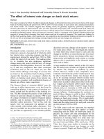
The graph in Figure 1 shows the CARs of the sampled
banks aggregated through all increase events, plotted
from day -15 to day 10 in our event window, a dura-
tion of 26 days. It can be seen that as the market an-
ticipates the change, this affects the value of the cumu-
lative abnormal returns. This may also reflect other
contemporaneous announcements and information
such as economic data supporting current expectations.
The early rise of the graph suggests that the market is
anticipating a positive impact from the cash rate an-
nouncement but corrects the magnitude of the return
once the actual announcement occurs.
CAR
0.000%
0.200%

0.400%
0.600%
0.800%
1.000%
1.200%
1.400%
1.600%
-15-13-11-9-7-5-3-1 1 3 5 7 9
Note: Shown above is the graph of financial firms abnormal returns graphed during event time on a day by day basis. The vertical
axis is the abnormal return in percentages and the horizontal axis days relative to the event day, 0 being event day.
Fig. 1. Banking firms' CARs during RBA increase events
Investment Management and Financial Innovations, Volume 5, Issue 4, 2008
232
We observe, consistent with Connolly and Kohler
(2004), that as a result of anticipation in the market,
there was an apparent increase in the cumulative ab-
normal returns up to 2 days prior to the event. How-
ever, once the rate is announced the market adjusts for
this information and the abnormal returns reduce to
reflect the value of information inherent in the an-
nouncement. In the days subsequent to the event, the
graph shows cumulative returns eased, losing any
gains made in abnormal return levels prior to the an-
nouncement; however, this net effect is not statistically
significant. CARs are however significant in the pre-
event period and the on-event period. The net positive
effect of at least 0.5 percent to 0.6 percent observed
during this period suggests a market value impact,
using the March 2005 event data, of $1.0 billion to
$1.2 billion for the banks studied. The overall impact,

looking at the full event window suggests no net-
negative impact on banking stock returns but rather a
net-positive short-term impact. We conclude that for
cash rate increases, contrary to the theory, we find that
cash rate increase announcements do not negatively
affect Australian bank stock returns in the short term
and reject H1 for rate increases.
We now examine the results for rate decrease events
reported in Panel B. The results for banking stocks, as
before, are summarized across all events which repre-
sent rate decrease or cash rate decreases events. A
summary of the CARs and related Z values accumu-
lated over event sub-periods is presented as before. We
can see that the CARs of banking stocks in the pre-
event period are significant at the 5 percent level and
prices react generally positively, as measured by the
abnormal returns to anticipated announced decreases
in the cash rate. This result is a positive abnormal re-
turn of +0.67 percent; namely strong pre-event antici-
pation by the market. Positive returns are continued
through the on-event period where we find an addi-
tional significant positive return of +0.39 percent. In
the post-event period returns reverse to marginally
negative but there is no significance in the Z value and
the magnitude is relatively small
1
. However, the CARs
for the total event period show a significant positive
effect on bank stock returns so we report a net positive
increase in the CARs of 0.99 percent.

Panel D of Table 3 reports the number of positive
CARs reported for each rate decrease event for each
bank. It can be observed that the overall proportion of
positive returns during the pre-event period, collec-
tively the pre-plus on-event period, the post-event
period and the overall event window is in excess of
50%. In the on-event period this falls to less than 50%
of events, however this was expected as the market
anticipates the effects given the transparent policy
environment, with information being absorbed in the
pre-event period and reflected in the price. So that it is
only unexpected changes that will result in large on-
event movements.
The graph in Figure 2 plots the CARs of the sampled
banks during rate decrease events for each day in the
event window. In a similar manner to rate increases,
there is an upward trend in the CARs very early in the
event period, albeit with some fluctuation, which stabi-
lizes as we approach the event. Again, it can be seen
that as the market anticipates the change, it has in-
creased the value of the cumulative abnormal returns
in anticipation of cash rate decreases. The early rises of
the CARs in the graph continue all the way past the
event day when it approaches +1.1 percent and then
oscillates at the levels reached on event day of about 1
percent and do not decline. This suggests the market
has expected cash rate decreases and, on confirmation,
the positive effect in abnormal returns is sustained
after the event day.
CAR

0.000%
0.200%
0.400%
0.600%
0.800%
1.000%
1.200%
-15-13-11-9-7-5-3-1 1 3 5 7 9
Note: This graph presents financial firms cumulative average abnormal returns graphed during event time on a day by day basis. The
vertical axis is the abnormal return in percentages and the horizontal axis days relative to the event day, 0 being event day.
Fig. 2. Banking firms' CARs during RBA decrease events
1

1
During the period from 1990 to 1993 there was consecutive interest rate reduction that followed an extremely volatile and high interest period when interest rates
reached record levels and the cash rate was in excess of 17.5 percent. The conclusions drawn in our analysis were not altered by the exclusion of these events.
Investment Management and Financial Innovations, Volume 5, Issue 4, 2008
233
Although the graph illustrates continuity of the posi-
tive CARs after the event day they are not significant
in the post event period. Interest rate reductions create
a favorable environment for the banking market, as
evident from the graph, supporting well established
theory and the experience of other markets that bank
stocks experience positive effects when cash rates are
decreased
1
. This represents a cumulative benefit of
approximately 0.9 percent for the overall event period
or 1.1 percent for the pre-event and post-event periods.

This reflects a market value impact, based on March
2005 data, of $1.6 billion to $2 billion.
We also undertook cross sectional regressions for
each of the pre-event, on-event and post-event peri-
ods to examine whether CARs reported varied due
to other effects such as size of firm. This was done
for rate increases and decreases. We have not re-
ported these regressions here as there was no sig-
nificance found in relation to the size of banking
firm as measured by total assets.
To enhance the robustness of our findings, given the
relatively small number of firms in our sample, we
have conducted the non-parametric generalized sign
test. The generalized sign test is of benefit to our
study as it does not require us to assume normality
in our data, although it does assume independence
between observations (Cowan and Sergeant, 1996).
The results are summarized in Table 4 below.
Table 4. Generalized sign test for positive abnormal
returns
Generalized sign test for positive cumulative abnormal returns
Est. period Event day Event per.
Positive returns 9682 39 51
Increases No. 19,200 96 96
Proportion 50.4% 40.6% 53.1%
Z value (1.92)* 0.53
Positive returns 15157 89 98
No. ARs 31,000 155 155
Decreases Proportion 48.9% 57.4% 63.2%
Z value 2.12** 3.57***

Notes: * significant at 10% level, ** significant at 5% level, ***
significant at 1% level. Reported above are the results of our
generalized sign test. The table shows a count of the observa-
tions used during each of the increase and decrease estimation
periods for cumulative returns to determine the expected pro-
portion of positive returns. This is then used as a bench mark to
test the count of the positive returns during the event period for
rate increase and decrease events.

1
During our testing of events, we noted that there were three situations that
were tested to ensure they did not distort our results. We refer to the Septem-
ber 11, 2001 and the period of 1990 to 1993 when there were 15 consecutive
decreases and two coincident CPI announcements. These circumstances
were examined to see if our results were altered by their exclusion. There
was no change in the conclusions drawn due to these circumstances.
In our test we look at the incidence of positive ab-
normal returns, and we can see from Table 4 that
our event period ARs for both increases and de-
creases indicate that our results are statistically sig-
nificant at the 10 percent and the 5 percent level.
However, we also report no significant support for
negative effects on stock returns in the overall event
period for increase events supporting our rejection
of H1 for increases but also providing strong evi-
dence to support the results for the decrease events.
We conclude the analysis of our results for banking
firms by observing that our first hypothesis H1 is
supported for rate decreases but not for increases.
We have demonstrated significant abnormal returns

during the pre-event period supporting our hypothe-
sis H2, that there will be significant abnormal re-
turns in the pre-event period, as markets anticipate
the impact of cash rate changes on banks stocks. We
also find sufficient evidence to empirically support
hypothesis H3 regarding asymmetrical effects. In-
creases and decreases have similar responses in the
pre-event period, symmetric responses in the on-
event period and inconclusive results in the post-
event sub-period.
4.2. Non financial firms. In Panel A of Table 5 we
report the impacts of rate increase events for non-
financial firms and again we present the cumulative
average abnormal returns and the corresponding Z
values, grouped by event sub-period and the event
period overall. We see that the reported CAR value
is -0.61 percent during the pre-event period. This
suggests a negative relationship with the rate change
however, the Z value fails to achieve significance at
the 10 percent level. In the on-event period how-
ever, we report a positive return of 0.13 percent
once again with no significance. In the post-event
period, we report a negative return of -0.53 percent
also with no significance. Therefore, we find no
significance in the CARs in any of the sub periods,
namely the pre-event, on-event and post-event peri-
ods somewhat consistent with the literature which
suggests non-financial firms are not impacted by
monetary policy, rate change announcements, in the
short term.

Table 5. Non-financial firms' event period CARs
Panel A. Non-financial firms – rate increases
Window CAR Z(CAR)
-15 to -2
Pre-event
-0.610% -1.596
-1 to +1
On-event
0.128% 0.317
+2 to +10
Post-event
-0.532% -1.433
-15 to 10
All event
-1.015% -1.820*
Investment Management and Financial Innovations, Volume 5, Issue 4, 2008
234
Table 5 (cont.). Non-financial firms' event period CARs
Panel B. Non-financial firms  rate decreases
Window CAR T (CAAR)
-15 to -2
Pre-event
-0.280% -1.218
-1 to +1
On-event
-0.015% -0.230
+2 to +10
Post-event
0.267% 1.182
-15 to 10

Total event
-0.028% -0.415
Notes: * significant at 10%, ** significant at 5%, *** significant at
1%. Panel A contains the cumulative CARs during rate increase
events for our sample non financial indices. The CARs are calculated
by accumulating the cross sectional average abnormal returns during
each event sub-period on a day by day basis into pre-event, on-event
and post-event sub-periods together with the associated Z scores. The
cross sectional abnormal returns are calculated by taking an average
for each event day across all sampled non-financial indices and across
all rate increase events on a day by day basis for each of the days in
the event window. Panel B contains non financial indices CAR data
during rate decreases calculated as for Panel A.
The graph in Figure 3 plots the cumulative aver-
age abnormal returns as before for non-financial
firms for rate increase events. We observe that the
results are not clear with respect to movement
through the event period. The graph starts with
negative returns and does not indicate a trend and
neither does it indicate possible anticipatory ef-
fects of the event. There are large movements of
the CAR line with oscillation at negative levels of
abnormal returns all the way through to the event
period. The CARs become increasingly negative
post-event, remain at around -0.4 percent and then
fall 3 days after the event. It is possible that non-
financial firms have a more significant lag effect
that is not observable in the event window. How-
ever, there is no reason to pursue this based on the
literature. Contrasting the results observed for

bank stocks, we find no significance in the ab-
normal returns of non-financial stock returns in
the on-event period due to RBA rate increase an-
nouncements.
Note: Shown above is the graph of non-financial firms abnormal returns graphed during event time on a day by day basis. The verti-
cal axis is the abnormal return in percentages and the horizontal axis days relative to the event day, 0 being event day.
Fig. 3. Non-financial firm CARs during RBA increase events
We now consider the impact of rate decrease events
for non-financial firms in Panel B of Table 5. We
find that decrease events show spurious results with
negative CARs in the pre-event and on-event peri-
ods and positive CARs on-event. In all cases the Z
values are not significant, and do not allow any con-
clusions to be drawn. Contrasting the pre- and on-
event sub-periods, the CARs for the post-event pe-
riod are positive but, again are not significant. Fig-
ure 4 below illustrates the movement of the cumula-
tive abnormal returns of the non-financial stocks
over the event days.
Note: This graph presents non-financial firms abnormal returns graphed during event time on a day by day basis. The vertical axis is
the abnormal return in percentages and the horizontal axis days relative to the event day, 0 being event day.
Fig. 4. Non-financial firms' CARs during RBA decrease events
Investment Management and Financial Innovations, Volume 5, Issue 4, 2008
235
We can see that the CARs start and finish at ap-
proximately the same point on the graph vertical
axis with enormous variations that in between, with
the CARs remaining negative throughout the event
window. There is an initial negative abnormal return
that increases as it approaches day 12, oscillates

between -0.2 and -0.4 percent, and gradually returns
back to its starting level. There are no anticipatory
effects evident as we approach the event day. The
graph suggests a negative CAR that eventually re-
turns back to original levels found at entry into the
event window, however as we have seen from Table
5 this is not statistically significant. We therefore
find that there is no significant impact on the stock
returns of non-financial firms in the event window
arising from RBA rate decrease announcements. We
therefore find support for hypothesis H4.
Conclusion
We undertook this study to examine the reaction of
bank stock returns to changes in the cash rate, as
measured by their abnormal and cumulative returns.
The results were obtained by examining the stock
returns of selected listed Australian banks, studied
as a group, representing in excess of 80 percent of
the market. We contrasted the response of these
stocks to those of non-financial firms using a selec-
tion of industry indices. These returns were exam-
ined for 10 rate increase events and 23 rate decrease
events affecting 10 banks using the well established
event study methodology. We find that, for rate
increase events, contrary to one well established
theory which suggests a negative relationship, bank
stocks report significant net-positive CARs in total
during the pre-event and on-event periods. We find
no significance in CARs for returns of the post-
event sub-period and therefore conclude that bank

stock returns in Australia are
not negatively im-
pacted in the short term, by cash rate increases. Cash
rate increases have a small positive short-term ef-
fect. This finding is inconsistent with the US litera-
ture. In the case of rate decreases, we found that
CARs for bank stocks are positive and significant in
both the pre-event and the on-event sub-periods.
RBA decreases in the cash rate target have a signifi-
cant and positive effect on bank stock returns con-
sistent with the established theory. We also analyzed
the effects of these returns on non-financial firms. In
the case of increases and decreases, there was no
significance in the abnormal returns of non-financial
firms for rate increases or decreases.
The positive impact on bank stock returns due to
rate increases needs to be considered in the context
of two perspectives: the market power of the domi-
nant banks and the economic environment. The
Australian economy has benefited from relatively
low inflation and interest rates. The majority of the
interest rate increases initiated by the RBA were to
control overheating of sectors in the economy to
prevent a boom bust cycle. Sectors such as housing
have boomed during the late 1990s and early 2000s
and the RBA tried to discourage what it regards as
the formation of large asset bubbles on the back of
strong demand for consumer debt.
References
1. APRA (2005). Australian Prudential Regulatory Authority  Monthly Banking Statistics. URL

Statistics/Monthly-Banking-Statistics.cfm
2. Beck, T., Demirguc-Kunt, A., Levine, R. (2003). Bank Concentration and Crises. National Bureau of Economic
Research, Inc, NBER Working Papers: 9921.
3. Berg, S.A., Kim, M. (1998). Banks as Multi-output Oligopolies: An Empirical Evaluation of the Retail and Corpo-
rate Banking Markets, Journal of Money, Credit, and Banking 30, 135-153.
4. Berger, A.N., Demirguc-Kunt, A., Levine, R., Haubrich, J.G. (2004). Bank Concentration and Competition: An
Evolution in the Making, Journal of Money, Credit, and Banking 36, 433-451.
5. Bernanke, B.S., Kuttner, K.N. (2005). What Explains the Stock Market's Reaction to Federal Reserve Policy, The
Journal of Finance 60, 1221-1257.
6. Bikker, J.A., Haaf, K. (2002). Competition, Concentration and Their Relationship: An Empirical Analysis of the
Banking Industry, Journal of Banking and Finance 26, 2191-2214.
7. Boehmer, E., Musumeci, J., Poulsen, A.B. (1991). Event-study methodology under conditions of event-induced
variance, Journal of Financial Economics 30, 253-272.
8. Brown, S.J., Warner, J.B. (1985). Using Daily Stock Returns - The Case of Event Studies, Journal of Financial
Economics 14, 3-31.
9. Campbell, J.Y., Lo, A.W., MacKinlay, A.C. (1997). The Econometrics of Financial Markets. Princeton, N.J.:
Princeton University Press, 1997.
10. Claessens, S., Laeven, L. (2004). What Drives Bank Competition? Some International Evidence, Journal of
Money, Credit & Banking 36, 563-583.
11. Connolly, E., Kohler, M. (2004). News and Interest rate expectations: A study of six central banks. Group E &
Australia. RBo (Eds.). Reserve Bank of Australia.
12. Cook, T., Hahn, T. (1989). The effect of changes in the federal funds rate target on market interest rates in the
1970s, Journal of Monetary Economics 24, 331-351.
13. Coppel, J., Connolly, E. (2003). What do Financial Market Data tell us about Monetary Policy transparency?
Group E & Australia. RBo (Eds.).
Investment Management and Financial Innovations, Volume 5, Issue 4, 2008
236
14. Cowan, A.R., Sergeant, A.M.A. (1996). Trading Frequency and Event Study Test Specification, Journal of Bank-
ing and Finance 20, 1731-1757.
15. Dennis, S.A., Jeffrey, A. (2002). Structural changes in Australian bank risk. 12, 1-17.

16. Diggle, J., Brooks, R. (2007). The target cash rate and its impact on investment asset returns in Australia, Applied
Financial Economics 17, 615-633.
17. Fama, E.F. (1970). Efficient Capital Markets: A review of Theory and Empircal Work, Journal of Finance 25, 383-417.
18. Fed (2006). US Federal Reserve
Insured US Chartered Commercial Banks that have Consolidated Assets of
$300M or more.
Board of Governors of the Federal Reserve System of the United States.
19. Flannery, M.J., James, C.M. (1984a). The Effect of Interest Rate Changes on the Common Stock Returns of Fi-
nancial Institutions, The Journal of Finance XXXIX, 1141-53.
20. Flannery, M.J., James, C.M. (1984b). Market Evidence on the Effective Maturity of Bank Assets and Liabilities,
Journal of Money, Credit & Banking 16, 435-445.
21. Gasbarro, D., Monroe, G.S. (2004). The impact of monetary policy candidness on Australian financial markets,
Journal of Multinational Financial Management 14, 35-46.
22. Gordon, M.J. (1962). The Investment, Financing, and Valuation of the Corporation. Richard D Irwin Inc., Homewood, IL.
23. Ho, T.S.Y., Saunders, A. (1981). The Determinants of Bank Interest Margins: Theory and Empirical Evidence,
The Journal of Financial and Quantitative Analysis 16, 581-600.
24. Hurley, W.J., Johnson, L.D. (1994). A Realistic Dividend Valuation Model. Financial Analysts Journal 50, 50-54.
25. Kim, S J., Nguyen, D.Q.T. (2008). The reaction of the Australian financial markets to the interest rate news from
the Reserve Bank of Australia and the U.S. Fed. Research in International Business and Finance 22, 378-395.
26. Kuttner, K.N. (2001). Monetary policy surprises and interest rates: Evidence from the Fed funds futures market,
Journal of Monetary Economics 47, 523-544.
27. Lintner, J. (1965). The Valuation of Risk Assets and the Selection of Risky Investments in Stock Portfolios and
Capital Budgets, The Review of Economic Statistics 47, 13-37.
28. Lowe, P. (1995). The Link Between the Cash Rate and Market Interest Rates. Department EA (Ed.). The Reserve
Bank of Australia.
29. Lynge, M.J., Zumwalt, K. (1980). An Empirical Study of The Interest Rate Sensitivity of Commercial Bank Re-
turns: A Multi-Index Approach, Journal of Financial and Quantitative Analysis 15, 731-742.
30. MacKinlay, A.C. (1997). Event Studies in Economics and Finance, Journal of Economic Literature XXXV, 13-39.
31. Madura, J., Schnusenberg, O. (2000). The Effect of Federal Reserve Policies on Bank Equity Returns, Journal of
Financial Research 23, 421-447.

32. RBA (2005). Reserve Bank of Australia URL
33. Ross, S.A. (1976). The Arbitrage Theory of Capital Asset Pricing, Journal of Economic Theory 13, 341-360.
34. Sharpe, W.F. (1964). Capital Asset Prices: A Theory of Market Equilibrium under Conditions of Risk, The Journal
of Finance 19, 425-442.
35. Sorensen, E.H., Williamson, D.A. (1985). Some Evidence on the Value of Dividend Discount Models, Financial
Analysts Journal 41, 60-69.
36. Stiglitz, J.E., Weiss, A. (1981). Credit Rationing in Markets with Imperfect Information, The American Economic
Review 71, 393-410.
37. Stone, B. (1974). Systematic Interest-rate Risk in a Two-index Model of Returns, Journal of Financial and Quanti-
tative Analysis 10, 709-721.
38. Strong, N. (1992). Modelling abnormal returns: A reveiw article, Journal of Business Finance and Accounting, 533-553.
39. Thorsten, B., Demirguc-Kunt, A., Ross, L. (2006). Bank concentration, competition, and crises: First results, Jour-
nal of Banking & Finance 30, 1581-1603.
40. Williams, B. (2002). Domestic and international determinants of bank profits: Foreign banks in Australia, Journal
of Banking and Finance 27, 1185-1210.
41. Williams, B. (2007). Factors Determining Net Interest Margins in Australia: Domestic and Foreign Banks, Finan-
cial Markets, Institutions & Instruments 16, 145-166.
42. Williams, J.B. (1956). The Theory of Investment Value, North-Holland Pub.Co., Amsterdam.