Báo cáo khoa học: "Efficient Tree-based Approximation for Entailment Graph Learning" doc

Proceedings of the 50th Annual Meeting of the Association for Computational Linguistics, pages 117–125,
Jeju, Republic of Korea, 8-14 July 2012.
c
2012 Association for Computational Linguistics
Efficient Tree-based Approximation for Entailment Graph Learning
Jonathan Berant
§
, Ido Dagan
†
, Meni Adler
†
, Jacob Goldberger
‡
§ The Blavatnik School of Computer Science, Tel Aviv University
† Department of Computer Science, Bar-Ilan University
‡ Faculty of Engineering, Bar-Ilan University

{dagan,goldbej}@{cs,eng}.biu.ac.il

Abstract
Learning entailment rules is fundamental in
many semantic-inference applications and has
been an active field of research in recent years.
In this paper we address the problem of learn-
ing transitive graphs that describe entailment
rules between predicates (termed entailment
graphs). We first identify that entailment
graphs exhibit a “tree-like” property and are
very similar to a novel type of graph termed
forest-reducible graph. We utilize this prop-
erty to develop an iterative efficient approxi-

mation algorithm for learning the graph edges,
where each iteration takes linear time. We
compare our approximation algorithm to a
recently-proposed state-of-the-art exact algo-
rithm and show that it is more efficient and
scalable both theoretically and empirically,
while its output quality is close to that given
by the optimal solution of the exact algorithm.
1 Introduction
Performing textual inference is in the heart of many
semantic inference applications such as Question
Answering (QA) and Information Extraction (IE). A
prominent generic paradigm for textual inference is
Textual Entailment (TUE) (Dagan et al., 2009). In
TUE, the goal is to recognize, given two text frag-
ments termed text and hypothesis, whether the hy-
pothesis can be inferred from the text. For example,
the text “Cyprus was invaded by the Ottoman Em-
pire in 1571” implies the hypothesis “The Ottomans
attacked Cyprus”.
Semantic inference applications such as QA and
IE crucially rely on entailment rules (Ravichandran
and Hovy, 2002; Shinyama and Sekine, 2006) or
equivalently inference rules, that is, rules that de-
scribe a directional inference relation between two
fragments of text. An important type of entailment
rule specifies the entailment relation between natu-
ral language predicates, e.g., the entailment rule ‘X
invade Y → X attack Y’ can be helpful in inferring
the aforementioned hypothesis. Consequently, sub-

stantial effort has been made to learn such rules (Lin
and Pantel, 2001; Sekine, 2005; Szpektor and Da-
gan, 2008; Schoenmackers et al., 2010).
Textual entailment is inherently a transitive rela-
tion , that is, the rules ‘x → y’ and ‘y → z’ imply
the rule ‘x → z’. Accordingly, Berant et al. (2010)
formulated the problem of learning entailment rules
as a graph optimization problem, where nodes are
predicates and edges represent entailment rules that
respect transitivity. Since finding the optimal set of
edges respecting transitivity is NP-hard, they em-
ployed Integer Linear Programming (ILP) to find the
exact solution. Indeed, they showed that applying
global transitivity constraints improves rule learning
comparing to methods that ignore graph structure.
More recently, Berant et al. (Berant et al., 2011) in-
troduced a more efficient exact algorithm, which de-
composes the graph into connected components and
then applies an ILP solver over each component.
Despite this progress, finding the exact solution
remains NP-hard – the authors themselves report
they were unable to solve some graphs of rather
moderate size and that the coverage of their method
is limited. Thus, scaling their algorithm to data sets
with tens of thousands of predicates (e.g., the extrac-
tions of Fader et al. (2011)) is unlikely.
117
In this paper we present a novel method for learn-
ing the edges of entailment graphs. Our method
computes much more efficiently an approximate so-

lution that is empirically almost as good as the exact
solution. To that end, we first (Section 3) conjecture
and empirically show that entailment graphs exhibit
a “tree-like” property, i.e., that they can be reduced
into a structure similar to a directed forest.
Then, we present in Section 4 our iterative ap-
proximation algorithm, where in each iteration a
node is removed and re-attached back to the graph in
a locally-optimal way. Combining this scheme with
our conjecture about the graph structure enables a
linear algorithm for node re-attachment. Section 5
shows empirically that this algorithm is by orders of
magnitude faster than the state-of-the-art exact al-
gorithm, and that though an optimal solution is not
guaranteed, the area under the precision-recall curve
drops by merely a point.
To conclude, the contribution of this paper is two-
fold: First, we define a novel modeling assumption
about the tree-like structure of entailment graphs and
demonstrate its validity. Second, we exploit this as-
sumption to develop a polynomial approximation al-
gorithm for learning entailment graphs that can scale
to much larger graphs than in the past. Finally, we
note that learning entailment graphs bears strong
similarities to related tasks such as Taxonomy In-
duction (Snow et al., 2006) and Ontology induction
(Poon and Domingos, 2010), and thus our approach
may improve scalability in these fields as well.
2 Background
Until recently, work on learning entailment rules be-

tween predicates considered each rule independently
of others and did not exploit global dependencies.
Most methods utilized the distributional similarity
hypothesis that states that semantically similar pred-
icates occur with similar arguments (Lin and Pan-
tel, 2001; Szpektor et al., 2004; Yates and Etzioni,
2009; Schoenmackers et al., 2010). Some meth-
ods extracted rules from lexicographic resources
such as WordNet (Szpektor and Dagan, 2009) or
FrameNet (Bob and Rambow, 2009; Ben Aharon et
al., 2010), and others assumed that semantic rela-
tions between predicates can be deduced from their
co-occurrence in a corpus via manually-constructed
patterns (Chklovski and Pantel, 2004).
Recently, Berant et al. (2010; 2011) formulated
the problem as the problem of learning global entail-
ment graphs. In entailment graphs, nodes are predi-
cates (e.g., ‘X attack Y’) and edges represent entail-
ment rules between them (‘X invade Y → X attack
Y’). For every pair of predicates i, j, an entailment
score w
ij
was learned by training a classifier over
distributional similarity features. A positive w
ij
in-
dicated that the classifier believes i → j and a nega-
tive w
ij
indicated that the classifier believes i  j.

Given the graph nodes V (corresponding to the pred-
icates) and the weighting function w : V × V → R,
they aim to find the edges of a graph G = (V, E)
that maximize the objective

(i,j)∈E
w
ij
under the
constraint that the graph is transitive (i.e., for every
node triplet (i, j, k), if (i, j) ∈ E and (j, k) ∈ E,
then (i, k) ∈ E).
Berant et al. proved that this optimization prob-
lem, which we term Max-Trans-Graph, is NP-hard,
and so described it as an Integer Linear Program
(ILP). Let x
ij
be a binary variable indicating the ex-
istence of an edge i → j in E. Then, X = {x
ij
:
i = j} are the variables of the following ILP for
Max-Trans-Graph:
arg max
X

i=j
w
ij
· x

ij
(1)
s.t. ∀
i,j,k∈V
x
ij
+ x
jk
− x
ik
≤ 1
∀
i,j∈V
x
ij
∈ {0, 1}
The objective function is the sum of weights over the
edges of G and the constraint x
ij
+ x
jk
− x
ik
≤ 1
on the binary variables enforces that whenever x
ij
=
x
jk
=1, then also x

ik
= 1 (transitivity).
Since ILP is NP-hard, applying an ILP solver di-
rectly does not scale well because the number of
variables is O(|V |
2
) and the number of constraints is
O(|V |
3
). Thus, even a graph with ∼80 nodes (predi-
cates) has more than half a million constraints. Con-
sequently, in (Berant et al., 2011), they proposed a
method that efficiently decomposes the graph into
smaller components and applies an ILP solver on
each component separately using a cutting-plane
procedure (Riedel and Clarke, 2006). Although this
method is exact and improves scalability, it does
not guarantee an efficient solution. When the graph
does not decompose into sufficiently small compo-
nents, and the weights generate many violations of
118
transitivity, solving Max-Trans-Graph becomes in-
tractable. To address this problem, we present in
this paper a method for approximating the optimal
set of edges within each component and show that
it is much more efficient and scalable both theoreti-
cally and empirically.
Do and Roth (2010) suggested a method for a re-
lated task of learning taxonomic relations between
terms. Given a pair of terms, a small graph is con-

structed and constraints are imposed on the graph
structure. Their work, however, is geared towards
scenarios where relations are determined on-the-fly
for a given pair of terms and no global knowledge
base is explicitly constructed. Thus, their method
easily produces solutions where global constraints,
such as transitivity, are violated.
Another approximation method that violates tran-
sitivity constraints is LP relaxation (Martins et al.,
2009). In LP relaxation, the constraint x
ij
∈ {0, 1}
is replaced by 0 ≤ x
ij
≤ 1, transforming the prob-
lem from an ILP to a Linear Program (LP), which
is polynomial. An LP solver is then applied on the
problem, and variables x
ij
that are assigned a frac-
tional value are rounded to their nearest integer and
so many violations of transitivity easily occur. The
solution when applying LP relaxation is not a transi-
tive graph, but nevertheless we show for comparison
in Section 5 that our method is much faster.
Last, we note that transitive relations have been
explored in adjacent fields such as Temporal Infor-
mation Extraction (Ling and Weld, 2010), Ontol-
ogy Induction (Poon and Domingos, 2010), and Co-
reference Resolution (Finkel and Manning, 2008).

3 Forest-reducible Graphs
The entailment relation, described by entailment
graphs, is typically from a “semantically-specific”
predicate to a more “general” one. Thus, intuitively,
the topology of an entailment graph is expected to be
“tree-like”. In this section we first formalize this in-
tuition and then empirically analyze its validity. This
property of entailment graphs is an interesting topo-
logical observation on its own, but also enables the
efficient approximation algorithm of Section 4.
For a directed edge i → j in a directed acyclic
graphs (DAG), we term the node i a child of node
j, and j a parent of i. A directed forest is a DAG
X
disease
be
epidemic in
Y
country
X
disease

common in
Y
country
X
disease

occur in
Y

country
X
disease

frequent in
Y
country
X
disease

begin in
Y
country
be epidemic in
common in
frequent in
occur in
begin in

be epidemic in
common in
frequent in
occur in
begin in

(a)
(b)
(c)
Figure 1: A fragment of an entailment graph (a), its SCC
graph (b) and its reduced graph (c). Nodes are predicates

with typed variables (see Section 5), which are omitted in
(b) and (c) for compactness.
where all nodes have no more than one parent.
The entailment graph in Figure 1a (subgraph from
the data set described in Section 5) is clearly not a
directed forest – it contains a cycle of size two com-
prising the nodes ‘X common in Y’ and ‘X frequent in
Y’, and in addition the node ‘X be epidemic in Y’ has
3 parents. However, we can convert it to a directed
forest by applying the following operations. Any
directed graph G can be converted into a Strongly-
Connected-Component (SCC) graph in the follow-
ing way: every strongly connected component (a set
of semantically-equivalent predicates, in our graphs)
is contracted into a single node, and an edge is added
from SCC S
1
to SCC S
2
if there is an edge in G from
some node in S
1
to some node in S
2
. The SCC graph
is always a DAG (Cormen et al., 2002), and if G is
transitive then the SCC graph is also transitive. The
graph in Figure 1b is the SCC graph of the one in
119
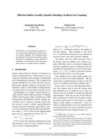
X

country
annex Y
place
X
country
invade Y
place
Y
place
be part of X
country


Figure 2: A fragment of an entailment graph that is not
an FRG.
Figure 1a, but is still not a directed forest since the
node ‘X be epidemic in Y’ has two parents.
The transitive closure of a directed graph G is
obtained by adding an edge from node i to node j
if there is a path in G from i to j. The transitive
reduction of G is obtained by removing all edges
whose absence does not affect its transitive closure.
In DAGs, the result of transitive reduction is unique
(Aho et al., 1972). We thus define the reduced graph
G
red
= (V
red
, E
red

) of a directed graph G as the
transitive reduction of its SCC graph. The graph in
Figure 1c is the reduced graph of the one in Fig-
ure 1a and is a directed forest. We say a graph is a
forest-reducible graph (FRG) if all nodes in its re-
duced form have no more than one parent.
We now hypothesize that entailment graphs are
FRGs. The intuition behind this assumption is
that the predicate on the left-hand-side of a uni-
directional entailment rule has a more specific mean-
ing than the one on the right-hand-side. For instance,
in Figure 1a ‘X be epidemic in Y’ (where ‘X’ is a type
of disease and ‘Y’ is a country) is more specific than
‘X common in Y’ and ‘X frequent in Y’, which are
equivalent, while ‘X occur in Y’ is even more gen-
eral. Accordingly, the reduced graph in Figure 1c
is an FRG. We note that this is not always the case:
for example, the entailment graph in Figure 2 is not
an FRG, because ‘X annex Y’ entails both ‘Y be part
of X’ and ‘X invade Y’, while the latter two do not
entail one another. However, we hypothesize that
this scenario is rather uncommon. Consequently, a
natural variant of the Max-Trans-Graph problem is
to restrict the required output graph of the optimiza-
tion problem (1) to an FRG. We term this problem
Max-Trans-Forest.
To test whether our hypothesis holds empirically
we performed the following analysis. We sampled
7 gold standard entailment graphs from the data set
described in Section 5, manually transformed them

into FRGs by deleting a minimal number of edges,
and measured recall over the set of edges in each
graph (precision is naturally 1.0, as we only delete
gold standard edges). The lowest recall value ob-
tained was 0.95, illustrating that deleting a very
small proportion of edges converts an entailment
graph into an FRG. Further support for the prac-
tical validity of this hypothesis is obtained from
our experiments in Section 5. In these experiments
we show that exactly solving Max-Trans-Graph and
Max-Trans-Forest (with an ILP solver) results in
nearly identical performance.
An ILP formulation for Max-Trans-Forest is sim-
ple – a transitive graph is an FRG if all nodes in
its reduced graph have no more than one parent. It
can be verified that this is equivalent to the following
statement: for every triplet of nodes i, j, k, if i → j
and i → k, then either j → k or k → j (or both).
Therefore, the ILP is formulated by adding this lin-
ear constraint to ILP (1):
∀
i,j,k∈V
x
ij
+x
ik
+(1 − x
jk
)+(1 − x
kj

) ≤ 3 (2)
We note that despite the restriction to FRGs, Max-
Trans-Forest is an NP-hard problem by a reduction
from the X3C problem (Garey and Johnson, 1979).
We omit the reduction details for brevity.
4 Sequential Approximation Algorithms
In this section we present Tree-Node-Fix, an efficient
approximation algorithm for Max-Trans-Forest, as
well as Graph-Node-Fix, an approximation for Max-
Trans-Graph.
4.1 Tree-Node-Fix
The scheme of Tree-Node-Fix (TNF) is the follow-
ing. First, an initial FRG is constructed, using some
initialization procedure. Then, at each iteration a
single node v is re-attached (see below) to the FRG
in a way that improves the objective function. This
is repeated until the value of the objective function
cannot be improved anymore by re-attaching a node.
Re-attaching a node v is performed by removing
v from the graph and connecting it back with a better
set of edges, while maintaining the constraint that it
is an FRG. This is done by considering all possible
edges from/to the other graph nodes and choosing
120
(a)
d
c
v …
c
v

c
d
1
…
d
2
v
…

…

…

r
1
r
2
v
(b) (b’) (c)
r
3
…

Figure 3: (a) Inserting v into a component c ∈ V
red
. (b)
Inserting v as a child of c and a parent of a subset of c’s
children in G
red
. (b’) A node d that is a descendant but

not a child of c can not choose v as a parent, as v becomes
its second parent. (c) Inserting v as a new root.
the optimal subset, while the rest of the graph re-
mains fixed. Formally, let S
v−in
=

i=v
w
iv
· x
iv
be the sum of scores over v’s incoming edges and
S
v−out
=

k=v
w
vk
· x
vk
be the sum of scores over
v’s outgoing edges. Re-attachment amounts to opti-
mizing a linear objective:
arg max
X
v
(S
v-in

+ S
v-out
) (3)
where the variables X
v
⊆ X are indicators for all
pairs of nodes involving v. We approximate a solu-
tion for (1) by iteratively optimizing the simpler ob-
jective (3). Clearly, at each re-attachment the value
of the objective function cannot decrease, since the
optimization algorithm considers the previous graph
as one of its candidate solutions.
We now show that re-attaching a node v is lin-
ear. To analyze v’s re-attachment, we consider the
structure of the directed forest G
red
just before v is
re-inserted, and examine the possibilities for v’s in-
sertion relative to that structure. We start by defin-
ing some helpful notations. Every node c ∈ V
red
is a connected component in G. Let v
c
∈ c be an
arbitrary representative node in c. We denote by
S
v-in
(c) the sum of weights from all nodes in c and
their descendants to v, and by S
v-out

(c) the sum of
weights from v to all nodes in c and their ancestors:
S
v-in
(c) =

i∈c
w
iv
+

k /∈c
w
kv
x
kv
c
S
v-out
(c) =

i∈c
w
vi
+

k /∈c
w
vk
x

v
c
k
Note that {x
v
c
k
, x
kv
c
} are edge indicators in G
and not G
red
. There are two possibilities for re-
attaching v – either it is inserted into an existing
component c ∈ V
red
(Figure 3a), or it forms a new
component. In the latter, there are also two cases:
either v is inserted as a child of a component c (Fig-
ure 3b), or not and then it becomes a root in G
red
(Figure 3c). We describe the details of these 3 cases:
Case 1: Inserting v into a component c ∈ V
red
.
In this case we add in G edges from all nodes in c
and their descendants to v and from v to all nodes in
c and their ancestors. The score (3) in this case is
s

1
(c)  S
v-in
(c) + S
v-out
(c) (4)
Case 2: Inserting v as a child of some c ∈ V
red
.
Once c is chosen as the parent of v, choosing v’s
children in G
red
is substantially constrained. A node
that is not a descendant of c can not become a child
of v, since this would create a new path from that
node to c and would require by transitivity to add a
corresponding directed edge to c (but all graph edges
not connecting v are fixed). Moreover, only a direct
child of c can choose v as a parent instead of c (Fig-
ure 3b), since for any other descendant of c, v would
become a second parent, and G
red
will no longer be
a directed forest (Figure 3b’). Thus, this case re-
quires adding in G edges from v to all nodes in c and
their ancestors, and also for each new child of v, de-
noted by d ∈ V
red
, we add edges from all nodes in
d and their descendants to v. Crucially, although the

number of possible subsets of c’s children in G
red
is
exponential, the fact that they are independent trees
in G
red
allows us to go over them one by one, and
decide for each one whether it will be a child of v
or not, depending on whether S
v-in
(d) is positive.
Therefore, the score (3) in this case is:
s
2
(c)  S
v-out
(c)+

d∈child(c)
max(0, S
v-in
(d)) (5)
where child(c) are the children of c.
Case 3: Inserting v as a new root in G
red
. Similar
to case 2, only roots of G
red
can become children of
v. In this case for each chosen root r we add in G

edges from the nodes in r and their descendants to
v. Again, each root can be examined independently.
Therefore, the score (3) of re-attaching v is:
s
3


r
max(0, S
v-in
(r)) (6)
where the summation is over the roots of G
red
.
It can be easily verified that S
v-in
(c) and
S
v-out
(c) satisfy the recursive definitions:
121
Algorithm 1 Computing optimal re-attachment
Input: FRG G = (V, E), function w, node v ∈ V
Output: optimal re-attachment of v
1: remove v and compute G
red
= (V
red
, E
red

).
2: for all c ∈ V
red
in post-order compute S
v-in
(c) (Eq.
7)
3: for all c ∈ V
red
in pre-order compute S
v-out
(c) (Eq.
8)
4: case 1: s
1
= max
c∈V
red
s
1
(c) (Eq. 4)
5: case 2: s
2
= max
c∈V
red
s
2
(c) (Eq. 5)
6: case 3: compute s

3
(Eq. 6)
7: re-attach v according to max(s
1
, s
2
, s
3
).
S
v-in
(c) =

i∈c
w
iv
+

d∈child(c)
S
v-in
(d), c ∈ V
red
(7)
S
v-out
(c) =

i∈c
w

vi
+ S
v-out
(p), c ∈ V
red
(8)
where p is the parent of c in G
red
. These recursive
definitions allow to compute in linear time S
v-in
(c)
and S
v-out
(c) for all c (given G
red
) using dynamic
programming, before going over the cases for re-
attaching v. S
v-in
(c) is computed going over V
red
leaves-to-root (post-order), and S
v-out
(c) is com-
puted going over V
red
root-to-leaves (pre-order).
Re-attachment is summarized in Algorithm 1.
Computing an SCC graph is linear (Cormen et al.,

2002) and it is easy to verify that transitive reduction
in FRGs is also linear (Line 1). Computing S
v-in
(c)
and S
v-out
(c) (Lines 2-3) is also linear, as explained.
Cases 1 and 3 are trivially linear and in case 2 we go
over the children of all nodes in V
red
. As the reduced
graph is a forest, this simply means going over all
nodes of V
red
, and so the entire algorithm is linear.
Since re-attachment is linear, re-attaching all
nodes is quadratic. Thus if we bound the number
of iterations over all nodes, the overall complexity is
quadratic. This is dramatically more efficient and
scalable than applying an ILP solver. In Section
5 we ran TNF until convergence and the maximal
number of iterations over graph nodes was 8.
4.2 Graph-node-fix
Next, we show Graph-Node-Fix (GNF), a similar
approximation that employs the same re-attachment
strategy but does not assume the graph is an FRG.
Thus, re-attachment of a node v is done with an
ILP solver. Nevertheless, the ILP in GNF is sim-
pler than (1), since we consider only candidate edges
v

i k
v
i k
v
i k
v
i k
Figure 4: Three types of transitivity constraint violations.
involving v. Figure 4 illustrates the three types of
possible transitivity constraint violations when re-
attaching v. The left side depicts a violation when
(i, k) /∈ E, expressed by the constraint in (9) below,
and the middle and right depict two violations when
the edge (i, k) ∈ E, expressed by the constraints
in (10). Thus, the ILP is formulated by adding the
following constraints to the objective function (3):
∀
i,k∈V \{v}
if (i, k) /∈ E, x
iv
+ x
vk
≤ 1 (9)
if (i, k) ∈ E, x
vi
≤ x
vk
, x
kv
≤ x

iv
(10)
x
iv
, x
vk
∈ {0, 1} (11)
Complexity is exponential due to the ILP solver;
however, the ILP size is reduced by an order of mag-
nitude to O(|V |) variables and O(|V |
2
) constraints.
4.3 Adding local constraints
For some pairs of predicates i, j we sometimes have
prior knowledge whether i entails j or not. We term
such pairs local constraints, and incorporate them
into the aforementioned algorithms in the following
way. In all algorithms that apply an ILP solver, we
add a constraint x
ij
= 1 if i entails j or x
ij
= 0 if i
does not entail j. Similarly, in TNF we incorporate
local constraints by setting w
ij
= ∞ or w
ij
= −∞.
5 Experiments and Results

In this section we empirically demonstrate that TNF
is more efficient than other baselines and its output
quality is close to that given by the optimal solution.
5.1 Experimental setting
In our experiments we utilize the data set released
by Berant et al. (2011). The data set contains 10 en-
tailment graphs, where graph nodes are typed pred-
icates. A typed predicate (e.g., ‘X
disease
occur in
Y
country
’) includes a predicate and two typed vari-
ables that specify the semantic type of the argu-
ments. For instance, the typed variable X
disease
can
be instantiated by arguments such as ‘flu’ or ‘dia-
betes’. The data set contains 39,012 potential edges,
122
of which 3,427 are annotated as edges (valid entail-
ment rules) and 35,585 are annotated as non-edges.
The data set also contains, for every pair of pred-
icates i, j in every graph, a local score s
ij
, which is
the output of a classifier trained over distributional
similarity features. A positive s
ij
indicates that the

classifier believes i → j. The weighting function for
the graph edges w is defined as w
ij
= s
ij
−λ, where
λ is a single parameter controlling graph sparseness:
as λ increases, w
ij
decreases and becomes nega-
tive for more pairs of predicates, rendering the graph
more sparse. In addition, the data set contains a set
of local constraints (see Section 4.3).
We implemented the following algorithms for
learning graph edges, where in all of them the graph
is first decomposed into components according to
Berant et al’s method, as explained in Section 2.
No-trans Local scores are used without transitiv-
ity constraints – an edge (i, j) is inserted iff w
ij
> 0.
Exact-graph Berant et al.’s exact method (2011)
for Max-Trans-Graph, which utilizes an ILP solver
1
.
Exact-forest Solving Max-Trans-Forest exactly
by applying an ILP solver (see Eq. 2).
LP-relax Solving Max-Trans-Graph approxi-
mately by applying LP-relaxation (see Section 2)
on each graph component. We apply the LP solver

within the same cutting-plane procedure as Exact-
graph to allow for a direct comparison. This also
keeps memory consumption manageable, as other-
wise all |V |
3
constraints must be explicitly encoded
into the LP. As mentioned, our goal is to present
a method for learning transitive graphs, while LP-
relax produces solutions that violate transitivity.
However, we run it on our data set to obtain empiri-
cal results, and to compare run-times against TNF.
Graph-Node-Fix (GNF) Initialization of each
component is performed in the following way: if the
graph is very sparse, i.e. λ ≥ C for some constant C
(set to 1 in our experiments), then solving the graph
exactly is not an issue and we use Exact-graph. Oth-
erwise, we initialize by applying Exact-graph in a
sparse configuration, i.e., λ = C.
Tree-Node-Fix (TNF) Initialization is done as in
GNF, except that if it generates a graph that is not an
FRG, it is corrected by a simple heuristic: for every
node in the reduced graph G
red
that has more than
1
We use the Gurobi optimization package in all experiments.
●
●
●
●

●
●
●
−0.8 −0.6 −0.4 −0.2 0.0
10 50 100 500 5000 50000
−lambda
sec
●
Exact−graph
LP−relax
GNF
TNF
Figure 5: Run-time in seconds for various −λ values.
one parent, we choose from its current parents the
single one whose SCC is composed of the largest
number of nodes in G.
We evaluate algorithms by comparing the set of
gold standard edges with the set of edges learned by
each algorithm. We measure recall, precision and
F
1
for various values of the sparseness parameter
λ, and compute the area under the precision-recall
Curve (AUC) generated. Efficiency is evaluated by
comparing run-times.
5.2 Results
We first focus on run-times and show that TNF is
efficient and has potential to scale to large data sets.
Figure 5 compares run-times
2

of Exact-graph,
GNF, TNF, and LP-relax as −λ increases and the
graph becomes denser. Note that the y-axis is in
logarithmic scale. Clearly, Exact-graph is extremely
slow and run-time increases quickly. For λ = 0.3
run-time was already 12 hours and we were unable
to obtain results for λ < 0.3, while in TNF we easily
got a solution for any λ. When λ = 0.6, where both
Exact-graph and TNF achieve best F
1
, TNF is 10
times faster than Exact-graph. When λ = 0.5, TNF
is 50 times faster than Exact-graph and so on. Most
importantly, run-time for GNF and TNF increases
much more slowly than for Exact-graph.
2
Run on a multi-core 2.5GHz server with 32GB of RAM.
123
0.0 0.1 0.2 0.3 0.4 0.5 0.6 0.7
0.0 0.2 0.4 0.6 0.8 1.0
recall
precision
●●●
●
●
●
●
●
●
●

●
●
●
●
●
●
●
●
●
●
●
●
●
●
Exact−graph
TNF
No−trans
Figure 6: Precision (y-axis) vs. recall (x-axis) curve.
Maximal F
1
on the curve is .43 for Exact-graph, .41 for
TNF, and .34 for No-trans. AUC in the recall range 0-0.5
is .32 for Exact-graph, .31 for TNF, and .26 for No-trans.
Run-time of LP-relax is also bad compared to
TNF and GNF. Run-time increases more slowly than
Exact-graph, but still very fast comparing to TNF.
When λ = 0.6, LP-relax is almost 10 times slower
than TNF, and when λ = −0.1, LP-relax is 200
times slower than TNF. This points to the difficulty
of scaling LP-relax to large graphs.

As for the quality of learned graphs, Figure 6 pro-
vides a precision-recall curve for Exact-graph, TNF
and No-trans (GNF and LP-relax are omitted from
the figure and described below to improve readabil-
ity). We observe that both Exact-graph and TNF
substantially outperform No-trans and that TNF’s
graph quality is only slightly lower than Exact-graph
(which is extremely slow). Following Berant et al.,
we report in the caption the maximal F
1
on the curve
and AUC in the recall range 0-0.5 (the widest range
for which we have results for all algorithms). Note
that compared to Exact-graph, TNF reduces AUC by
a point and the maximal F
1
score by 2 points only.
GNF results are almost identical to those of TNF
(maximal F
1
=0.41, AUC: 0.31), and in fact for all
λ configurations TNF outperforms GNF by no more
than one F
1
point. As for LP-relax, results are just
slightly lower than Exact-graph (maximal F
1
: 0.43,
AUC: 0.32), but its output is not a transitive graph,
and as shown above run-time is quite slow. Last, we

note that the results of Exact-forest are almost iden-
tical to Exact-graph (maximal F
1
: 0.43), illustrating
that assuming that entailment graphs are FRGs (Sec-
tion 3) is reasonable in this data set.
To conclude, TNF learns transitive entailment
graphs of good quality much faster than Exact-
graph. Our experiment utilized an available data
set of moderate size; However, we expect TNF to
scale to large data sets (that are currently unavail-
able), where other baselines would be impractical.
6 Conclusion
Learning large and accurate resources of entailment
rules is essential in many semantic inference appli-
cations. Employing transitivity has been shown to
improve rule learning, but raises issues of efficiency
and scalability.
The first contribution of this paper is a novel mod-
eling assumption that entailment graphs are very
similar to FRGs, which is analyzed and validated
empirically. The main contribution of the paper is
an efficient polynomial approximation algorithm for
learning entailment rules, which is based on this
assumption. We demonstrate empirically that our
method is by orders of magnitude faster than the
state-of-the-art exact algorithm, but still produces an
output that is almost as good as the optimal solution.
We suggest our method as an important step to-
wards scalable acquisition of precise entailment re-

sources. In future work, we aim to evaluate TNF on
large graphs that are automatically generated from
huge corpora. This of course requires substantial ef-
forts of pre-processing and test-set annotation. We
also plan to examine the benefit of TNF in learning
similar structures, e.g., taxonomies or ontologies.
Acknowledgments
This work was partially supported by the Israel
Science Foundation grant 1112/08, the PASCAL-
2 Network of Excellence of the European Com-
munity FP7-ICT-2007-1-216886, and the Euro-
pean Community’s Seventh Framework Programme
(FP7/2007-2013) under grant agreement no. 287923
(EXCITEMENT). The first author has carried out
this research in partial fulfilment of the requirements
for the Ph.D. degree.
124
References
Alfred V. Aho, Michael R. Garey, and Jeffrey D. Ullman.
1972. The transitive reduction of a directed graph.
SIAM Journal on Computing, 1(2):131–137.
Roni Ben Aharon, Idan Szpektor, and Ido Dagan. 2010.
Generating entailment rules from framenet. In Pro-
ceedings of the 48th Annual Meeting of the Association
for Computational Linguistics.
Jonathan Berant, Ido Dagan, and Jacob Goldberger.
2010. Global learning of focused entailment graphs.
In Proceedings of the 48th Annual Meeting of the As-
sociation for Computational Linguistics.
Jonathan Berant, Ido Dagan, and Jacob Goldberger.

2011. Global learning of typed entailment rules. In
Proceedings of the 49th Annual Meeting of the Associ-
ation for Computational Linguistics.
Coyne Bob and Owen Rambow. 2009. Lexpar: A freely
available english paraphrase lexicon automatically ex-
tracted from framenet. In Proceedings of IEEE Inter-
national Conference on Semantic Computing.
Timothy Chklovski and Patrick Pantel. 2004. Verb
ocean: Mining the web for fine-grained semantic verb
relations. In Proceedings of Empirical Methods in
Natural Language Processing.
Thomas H. Cormen, Charles E. leiserson, Ronald L.
Rivest, and Clifford Stein. 2002. Introduction to Al-
gorithms. The MIT Press.
Ido Dagan, Bill Dolan, Bernardo Magnini, and Dan Roth.
2009. Recognizing textual entailment: Rational, eval-
uation and approaches. Natural Language Engineer-
ing, 15(4):1–17.
Quang Do and Dan Roth. 2010. Constraints based tax-
onomic relation classification. In Proceedings of Em-
pirical Methods in Natural Language Processing.
Anthony Fader, Stephen Soderland, and Oren Etzioni.
2011. Identifying relations for open information ex-
traction. In Proceedings of Empirical Methods in Nat-
ural Language Processing.
J. R. Finkel and C. D. Manning. 2008. Enforcing transi-
tivity in coreference resolution. In Proceedings of the
46th Annual Meeting of the Association for Computa-
tional Linguistics.
Michael R. Garey and David S. Johnson. 1979. Comput-

ers and Intractability: A Guide to the Theory of NP-
Completeness. W. H. Freeman.
Dekang Lin and Patrick Pantel. 2001. Discovery of infer-
ence rules for question answering. Natural Language
Engineering, 7(4):343–360.
Xiao Ling and Dan S. Weld. 2010. Temporal informa-
tion extraction. In Proceedings of the 24th AAAI Con-
ference on Artificial Intelligence.
Andre Martins, Noah Smith, and Eric Xing. 2009. Con-
cise integer linear programming formulations for de-
pendency parsing. In Proceedings of the 47th Annual
Meeting of the Association for Computational Linguis-
tics.
Hoifung Poon and Pedro Domingos. 2010. Unsuper-
vised ontology induction from text. In Proceedings of
the 48th Annual Meeting of the Association for Com-
putational Linguistics.
Deepak Ravichandran and Eduard Hovy. 2002. Learning
surface text patterns for a question answering system.
In Proceedings of the 40th Annual Meeting of the As-
sociation for Computational Linguistics.
Sebastian Riedel and James Clarke. 2006. Incremental
integer linear programming for non-projective depen-
dency parsing. In Proceedings of Empirical Methods
in Natural Language Processing.
Stefan Schoenmackers, Jesse Davis, Oren Etzioni, and
Daniel S. Weld. 2010. Learning first-order horn
clauses from web text. In Proceedings of Empirical
Methods in Natural Language Processing.
Satoshi Sekine. 2005. Automatic paraphrase discovery

based on context and keywords between ne pairs. In
Proceedings of IWP.
Yusuke Shinyama and Satoshi Sekine. 2006. Preemptive
information extraction using unrestricted relation dis-
covery. In Proceedings of the Human Language Tech-
nology Conference of the NAACL, Main Conference.
Rion Snow, Dan Jurafsky, and Andrew Y. Ng. 2006.
Semantic taxonomy induction from heterogenous ev-
idence. In Proceedings of the 44th Annual Meeting of
the Association for Computational Linguistics.
Idan Szpektor and Ido Dagan. 2008. Learning entail-
ment rules for unary templates. In Proceedings of the
22nd International Conference on Computational Lin-
guistics.
Idan Szpektor and Ido Dagan. 2009. Augmenting
wordnet-based inference with argument mapping. In
Proceedings of TextInfer.
Idan Szpektor, Hristo Tanev, Ido Dagan, and Bonaven-
tura Coppola. 2004. Scaling web-based acquisition
of entailment relations. In Proceedings of Empirical
Methods in Natural Language Processing.
Alexander Yates and Oren Etzioni. 2009. Unsupervised
methods for determining object and relation synonyms
on the web. Journal of Artificial Intelligence Research,
34:255–296.
125