Báo cáo khoa học: "Efficient Inference Through Cascades of Weighted Tree Transducers" ppt

Proceedings of the 48th Annual Meeting of the Association for Computational Linguistics, pages 1058–1066,
Uppsala, Sweden, 11-16 July 2010.
c
2010 Association for Computational Linguistics
Efficient Inference Through Cascades of Weighted Tree Transducers
Jonathan May and Kevin Knight
Information Sciences Institute
University of Southern California
Marina del Rey, CA 90292
{jonmay,knight}@isi.edu
Heiko Vogler
Technische Universit
¨
at Dresden
Institut f
¨
ur Theoretische Informatik
01062 Dresden, Germany

Abstract
Weighted tree transducers have been pro-
posed as useful formal models for rep-
resenting syntactic natural language pro-
cessing applications, but there has been
little description of inference algorithms
for these automata beyond formal founda-
tions. We give a detailed description of
algorithms for application of cascades of
weighted tree transducers to weighted tree
acceptors, connecting formal theory with
actual practice. Additionally, we present

novel on-the-fly variants of these algo-
rithms, and compare their performance
on a syntax machine translation cascade
based on (Yamada and Knight, 2001).
1 Motivation
Weighted finite-state transducers have found re-
cent favor as models of natural language (Mohri,
1997). In order to make actual use of systems built
with these formalisms we must first calculate the
set of possible weighted outputs allowed by the
transducer given some input, which we call for-
ward application, or the set of possible weighted
inputs given some output, which we call backward
application. After application we can do some in-
ference on this result, such as determining its k
highest weighted elements.
We may also want to divide up our problems
into manageable chunks, each represented by a
transducer. As noted by Woods (1980), it is eas-
ier for designers to write several small transduc-
ers where each performs a simple transformation,
rather than painstakingly construct a single com-
plicated device. We would like to know, then,
the result of transformation of input or output by
a cascade of transducers, one operating after the
other. As we will see, there are various strate-
gies for approaching this problem. We will con-
sider offline composition, bucket brigade applica-
tion, and on-the-fly application.
Application of cascades of weighted string

transducers (WSTs) has been well-studied (Mohri,
1997). Less well-studied but of more recent in-
terest is application of cascades of weighted tree
transducers (WTTs). We tackle application of WTT
cascades in this work, presenting:
• explicit algorithms for application of WTT cas-
cades
• novel algorithms for on-the-fly application of
WTT cascades, and
• experiments comparing the performance of
these algorithms.
2 Strategies for the string case
Before we discuss application of WTTs, it is help-
ful to recall the solution to this problem in the WST
domain. We recall previous formal presentations
of WSTs (Mohri, 1997) and note informally that
they may be represented as directed graphs with
designated start and end states and edges labeled
with input symbols, output symbols, and weights.
1
Fortunately, the solution for WSTs is practically
trivial—we achieve application through a series
of embedding, composition, and projection oper-
ations. Embedding is simply the act of represent-
ing a string or regular string language as an iden-
tity WST. Composition of WSTs, that is, generat-
ing a single WST that captures the transformations
of two input WSTs used in sequence, is not at all
trivial, but has been well covered in, e.g., (Mohri,
2009), where directly implementable algorithms

can be found. Finally, projection is another triv-
ial operation—the domain or range language can
be obtained from a WST by ignoring the output or
input symbols, respectively, on its arcs, and sum-
ming weights on otherwise identical arcs. By em-
bedding an input, composing the result with the
given WST, and projecting the result, forward ap-
plication is accomplished.
2
We are then left with
a weighted string acceptor (WSA), essentially a
weighted, labeled graph, which can be traversed
1
We assume throughout this paper that weights are in
R
+
∪ {+∞}, that the weight of a path is calculated as the
product of the weights of its edges, and that the weight of a
(not necessarily finite) set T of paths is calculated as the sum
of the weights of the paths of T .
2
For backward applications, the roles of input and output
are simply exchanged.
1058
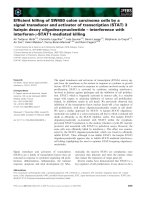
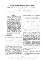
(a) Input string “a a” embedded in an
identity WST
(b) first WST in cascade (c) second WST in cascade
(d) Offline composition approach:
Compose the transducers
(e) Bucket brigade approach:

Apply WST (b) to WST (a)
(f) Result of offline or bucket application
after projection
(g) Initial on-the-fly
stand-in for (f)
(h) On-the-fly stand-in after exploring
outgoing edges of state ADF
(i) On-the-fly stand-in after best path has been found
Figure 1: Three different approaches to application through cascades of WSTs.
by well-known algorithms to efficiently find the k-
best paths.
Because WSTs can be freely composed, extend-
ing application to operate on a cascade of WSTs
is fairly trivial. The only question is one of com-
position order: whether to initially compose the
cascade into a single transducer (an approach we
call offline composition) or to compose the initial
embedding with the first transducer, trim useless
states, compose the result with the second, and so
on (an approach we call bucket brigade). The ap-
propriate strategy generally depends on the struc-
ture of the individual transducers.
A third approach builds the result incrementally,
as dictated by some algorithm that requests in-
formation about it. Such an approach, which we
call on-the-fly, was described in (Pereira and Ri-
ley, 1997; Mohri, 2009; Mohri et al., 2000). If
we can efficiently calculate the outgoing edges of
a state of the result WSA on demand, without cal-
culating all edges in the entire machine, we can

maintain a stand-in for the result structure, a ma-
chine consisting at first of only the start state of
the true result. As a calling algorithm (e.g., an im-
plementation of Dijkstra’s algorithm) requests in-
formation about the result graph, such as the set of
outgoing edges from a state, we replace the current
stand-in with a richer version by adding the result
of the request. The on-the-fly approach has a dis-
tinct advantage over the other two methods in that
the entire result graph need not be built. A graphi-
cal representation of all three methods is presented
in Figure 1.
3 Application of tree transducers
Now let us revisit these strategies in the setting
of trees and tree transducers. Imagine we have a
tree or set of trees as input that can be represented
as a weighted regular tree grammar
3
(WRTG) and
a WTT that can transform that input with some
weight. We would like to know the k-best trees the
WTT can produce as output for that input, along
with their weights. We already know of several
methods for acquiring k-best trees from a WRTG
(Huang and Chiang, 2005; Pauls and Klein, 2009),
so we then must ask if, analogously to the string
case, WTTs preserve recognizability
4
and we can
form an application WRTG. Before we begin, how-

ever, we must define WTTs and WRTGs.
3.1 Preliminaries
5
A ranked alphabet is a finite set Σ such that ev-
ery member σ ∈ Σ has a rank rk(σ) ∈ N. We
call Σ
(k)
⊆ Σ, k ∈ N the set of those σ ∈ Σ
such that rk(σ) = k. The set of variables is de-
noted X = {x
1
, x
2
, . . .} and is assumed to be dis-
joint from any ranked alphabet used in this paper.
We use ⊥ to denote a symbol of rank 0 that is not
in any ranked alphabet used in this paper. A tree
t ∈ T
Σ
is denoted σ(t
1
, . . . , t
k
) where k ≥ 0,
σ ∈ Σ
(k)
, and t
1
, . . . , t
k

∈ T
Σ
. For σ ∈ Σ
(0)
we
3
This generates the same class of weighted tree languages
as weighted tree automata, the direct analogue of WSAs, and
is more useful for our purposes.
4
A weighted tree language is recognizable iff it can be
represented by a wrtg.
5
The following formal definitions and notations are
needed for understanding and reimplementation of the pre-
sented algorithms, but can be safely skipped on first reading
and consulted when encountering an unfamiliar term.
1059
write σ ∈ T
Σ
as shorthand for σ(). For every set
S disjoint from Σ, let T
Σ
(S) = T
Σ∪S
, where, for
all s ∈ S, rk(s) = 0.
We define the positions of a tree
t = σ(t
1

, . . . , t
k
), for k ≥ 0, σ ∈ Σ
(k)
,
t
1
, . . . , t
k
∈ T
Σ
, as a set pos(t) ⊂ N
∗
such that
pos(t) = {ε} ∪ {iv | 1 ≤ i ≤ k, v ∈ pos(t
i
)}.
The set of leaf positions lv(t) ⊆ pos(t) are those
positions v ∈ pos(t) such that for no i ∈ N,
vi ∈ pos(t). We presume standard lexicographic
orderings < and ≤ on pos.
Let t, s ∈ T
Σ
and v ∈ pos(t). The label of t
at position v, denoted by t(v), the subtree of t at
v, denoted by t|
v
, and the replacement at v by s,
denoted by t[s]
v

, are defined as follows:
1. For every σ ∈ Σ
(0)
, σ(ε) = σ, σ|
ε
= σ, and
σ[s]
ε
= s.
2. For every t = σ(t
1
, . . . , t
k
) such that
k = rk(σ) and k ≥ 1, t(ε) = σ, t|
ε
= t,
and t[s]
ε
= s. For every 1 ≤ i ≤ k and
v ∈ pos(t
i
), t(iv) = t
i
(v), t|
iv
= t
i
|
v

, and
t[s]
iv
= σ(t
1
, . . . , t
i−1
, t
i
[s]
v
, t
i+1
, . . . , t
k
).
The size of a tree t, size(t) is |pos(t)|, the car-
dinality of its position set. The yield set of a tree
is the set of labels of its leaves: for a tree t, yd (t)
= {t(v) | v ∈ lv(t)}.
Let A and B be sets. Let ϕ : A → T
Σ
(B)
be a mapping. We extend ϕ to the mapping
ϕ :
T
Σ
(A) → T
Σ
(B) such that for a ∈A, ϕ(a) = ϕ(a)

and for k ≥ 0, σ ∈ Σ
(k)
, and t
1
, . . . , t
k
∈ T
Σ
(A),
ϕ(σ(t
1
, . . . , t
k
)) = σ(ϕ(t
1
), . . . , ϕ(t
k
)). We indi-
cate such extensions by describing ϕ as a substi-
tution mapping and then using ϕ without further
comment.
We use R
+
to denote the set {w ∈ R | w ≥ 0}
and R
∞
+
to denote R
+
∪ {+∞}.

Definition 3.1 (cf. (Alexandrakis and Bozapa-
lidis, 1987)) A weighted regular tree grammar
(WRTG) is a 4-tuple G = (N, Σ, P, n
0
) where:
1. N is a finite set of nonterminals, with n
0
∈ N
the start nonterminal.
2. Σ is a ranked alphabet of input symbols, where
Σ ∩ N = ∅.
3. P is a tuple (P

, π), where P

is a finite set
of productions, each production p of the form
n −→ u, n ∈ N , u ∈ T
Σ
(N), and π : P

→ R
+
is a weight function of the productions. We will
refer to P as a finite set of weighted produc-
tions, each production p of the form n
π(p)
−−→ u.
A production p is a chain production if it is
of the form n

i
w
−→ n
j
, where n
i
, n
j
∈ N.
6
6
In (Alexandrakis and Bozapalidis, 1987), chain produc-
tions are forbidden in order to avoid infinite summations. We
explicitly allow such summations.
A WR TG G is in normal form if each produc-
tion is either a chain production or is of the
form n
w
−→ σ(n
1
, . . . , n
k
) where σ ∈ Σ
(k)
and
n
1
, . . . , n
k
∈ N .

For WRTG G = (N, Σ, P, n
0
), s, t, u ∈ T
Σ
(N),
n ∈ N , and p ∈ P of the form n
w
−→ u, we
obtain a derivation step from s to t by replacing
some leaf nonterminal in s labeled n with u. For-
mally, s ⇒
p
G
t if there exists some v ∈ lv(s)
such that s(v) = n and s[u]
v
= t. We say this
derivation step is leftmost if, for all v

∈ lv(s)
where v

< v, s(v

) ∈ Σ. We henceforth as-
sume all derivation steps are leftmost. If, for
some m ∈ N, p
i
∈ P , and t
i

∈ T
Σ
(N) for all
1 ≤ i ≤ m, n
0
⇒
p
1
t
1
. . . ⇒
p
m
t
m
, we say
the sequence d = (p
1
, . . . , p
m
) is a derivation
of t
m
in G and that n
0
⇒
∗
t
m
; the weight of d

is wt(d) = π(p
1
) · . . . · π(p
m
). The weighted
tree language recognized by G is the mapping
L
G
: T
Σ
→ R
∞
+
such that for every t ∈ T
Σ
, L
G
(t)
is the sum of the weights of all (possibly infinitely
many) derivations of t in G. A weighted tree lan-
guage f : T
Σ
→ R
∞
+
is recognizable if there is a
WRTG G such that f = L
G
.
We define a partial ordering  on WRTGs

such that for WRTGs G
1
= (N
1
, Σ, P
1
, n
0
) and
G
2
= (N
2
, Σ, P
2
, n
0
), we say G
1
 G
2
iff
N
1
⊆ N
2
and P
1
⊆ P
2

, where the weights are
preserved.
Definition 3.2 (cf. Def. 1 of (Maletti, 2008))
A weighted extended top-down tree transducer
(WXTT) is a 5-tuple M = (Q, Σ, ∆, R, q
0
) where:
1. Q is a finite set of states.
2. Σ and ∆ are the ranked alphabets of in-
put and output symbols, respectively, where
(Σ ∪ ∆) ∩ Q = ∅.
3. R is a tuple (R

, π), where R

is a finite set
of rules, each rule r of the form q.y −→ u for
q ∈ Q, y ∈ T
Σ
(X), and u ∈ T
∆
(Q × X).
We further require that no variable x ∈ X ap-
pears more than once in y, and that each vari-
able appearing in u is also in y. Moreover,
π : R

→ R
∞
+

is a weight function of the
rules. As for WRTGs, we refer to R as a finite
set of weighted rules, each rule r of the form
q.y
π(r)
−−→ u.
A WXTT is linear (respectively, nondeleting)
if, for each rule r of the form q.y
w
−→ u, each
x ∈ yd (y) ∩ X appears at most once (respec-
tively, at least once) in u. We denote the class
of all WXTTs as wxT and add the letters L and N
to signify the subclasses of linear and nondeleting
WTT, respectively. Additionally, if y is of the form
σ(x
1
, . . . , x
k
), we remove the letter “x” to signify
1060
the transducer is not extended (i.e., it is a “tradi-
tional” WTT (F
¨
ul
¨
op and Vogler, 2009)).
For WXTT M = (Q, Σ, ∆, R, q
0
), s, t ∈ T

∆
(Q
× T
Σ
), and r ∈ R of the form q.y
w
−→ u, we obtain
a derivation step from s to t by replacing some
leaf of s labeled with q and a tree matching y by a
transformation of u, where each instance of a vari-
able has been replaced by a corresponding subtree
of the y-matching tree. Formally, s ⇒
r
M
t if there
is a position v ∈ pos(s), a substitution mapping
ϕ : X → T
Σ
, and a rule q.y
w
−→ u ∈ R such that
s(v) = (q,
ϕ(y)) and t = s[ϕ

(u)]
v
, where ϕ

is
a substitution mapping Q × X → T

∆
(Q × T
Σ
)
defined such that ϕ

(q

, x) = (q

, ϕ(x)) for all
q

∈ Q and x ∈ X. We say this derivation step
is leftmost if, for all v

∈ lv(s) where v

< v,
s(v

) ∈ ∆. We henceforth assume all derivation
steps are leftmost. If, for some s ∈ T
Σ
, m ∈ N,
r
i
∈ R, and t
i
∈ T

∆
(Q ×T
Σ
) for all 1 ≤ i ≤ m,
(q
0
, s) ⇒
r
1
t
1
. . . ⇒
r
m
t
m
, we say the sequence
d = (r
1
, . . . , r
m
) is a derivation of (s, t
m
) in M;
the weight of d is wt(d) = π(r
1
) · . . . · π(r
m
).
The weighted tree transformation recognized by

M is the mapping τ
M
: T
Σ
× T
∆
→ R
∞
+
, such
that for every s ∈ T
Σ
and t ∈ T
∆
, τ
M
(s, t) is the
sum of the weights of all (possibly infinitely many)
derivations of (s, t) in M . The composition of two
weighted tree transformations τ : T
Σ
×T
∆
→ R
∞
+
and µ : T
∆
×T
Γ

→ R
∞
+
is the weighted tree trans-
formation (τ; µ) : T
Σ
×T
Γ
→R
∞
+
where for every
s ∈ T
Σ
and u ∈ T
Γ
, (τ ; µ)(s, u) =

t∈T
∆
τ(s, t)
· µ(t, u).
3.2 Applicable classes
We now consider transducer classes where recog-
nizability is preserved under application. Table 1
presents known results for the top-down tree trans-
ducer classes described in Section 3.1. Unlike
the string case, preservation of recognizability is
not universal or symmetric. This is important for
us, because we can only construct an application

WRTG, i.e., a WRTG representing the result of ap-
plication, if we can ensure that the language gen-
erated by application is in fact recognizable. Of
the types under consideration, only wxLNT and
wLNT preserve forward recognizability. The two
classes marked as open questions and the other
classes, which are superclasses of wNT, do not or
are presumed not to. All subclasses of wxLT pre-
serve backward recognizability.
7
We do not con-
sider cases where recognizability is not preserved
in the remainder of this paper. If a transducer M
of a class that preserves forward recognizability is
applied to a WRTG G, we can call the forward ap-
7
Note that the introduction of weights limits recognizabil-
ity preservation considerably. For example, (unweighted) xT
preserves backward recognizability.
plication WR TG M(G)

and if M preserves back-
ward recognizability, we can call the backward ap-
plication WRTG M (G)

.
Now that we have explained the application
problem in the context of weighted tree transduc-
ers and determined the classes for which applica-
tion is possible, let us consider how to build for-

ward and backward application W RTGs. Our ba-
sic approach mimics that taken for WSTs by us-
ing an embed-compose-project strategy. As in
string world, if we can embed the input in a trans-
ducer, compose with the given transducer, and
project the result, we can obtain the application
WRTG. Embedding a WRTG in a wLNT is a triv-
ial operation—if the WRTG is in normal form and
chain production-free,
8
for every production of the
form n
w
−→ σ(n
1
, . . . , n
k
), create a rule of the form
n.σ(x
1
, . . . , x
k
)
w
−→ σ(n
1
.x
1
, . . . , n
k

.x
k
). Range
projection of a wxLNT is also trivial—for every
q ∈ Q and u ∈ T
∆
(Q × X) create a production
of the form q
w
−→ u

where u

is formed from u
by replacing all leaves of the form q.x with the
leaf q, i.e., removing references to variables, and
w is the sum of the weights of all rules of the form
q.y −→ u in R.
9
Domain projection for wxLT is
best explained by way of example. The left side of
a rule is preserved, with variables leaves replaced
by their associated states from the right side. So,
the rule q
1
.σ(γ(x
1
), x
2
)

w
−→ δ(q
2
.x
2
, β(α, q
3
.x
1
))
would yield the production q
1
w
−→ σ(γ(q
3
), q
2
) in
the domain projection. However, a deleting rule
such as q
1
.σ(x
1
, x
2
)
w
−→ γ(q
2
.x

2
) necessitates the
introduction of a new nonterminal ⊥ that can gen-
erate all of T
Σ
with weight 1.
The only missing piece in our embed-compose-
project strategy is composition. Algorithm 1,
which is based on the declarative construction of
Maletti (2006), generates the syntactic composi-
tion of a wxLT and a wLNT, a generalization
of the basic composition construction of Baker
(1979). It calls Algorithm 2, which determines
the sequences of rules in the second transducer
that match the right side of a single rule in the
first transducer. Since the embedded WRTG is of
type wLNT, it may be either the first or second
argument provided to Algorithm 1, depending on
whether the application is forward or backward.
We can thus use the embed-compose-project strat-
egy for forward application of wLNT and back-
ward application of wxLT and wxLNT. Note that
we cannot use this strategy for forward applica-
8
Without loss of generality we assume this is so, since
standard algorithms exist to remove chain productions
(Kuich, 1998;
´
Esik and Kuich, 2003; Mohri, 2009) and con-
vert into normal form (Alexandrakis and Bozapalidis, 1987).

9
Finitely many such productions may be formed.
1061
tion of wxLNT, even though that class preserves
recognizability.
Algorithm 1 COMPOSE
1: inputs
2: wxLT M
1
= (Q
1
, Σ, ∆, R
1
, q
1
0
)
3: wLNT M
2
= (Q
2
, ∆, Γ, R
2
, q
2
0
)
4: outputs
5: wxLT M
3

= ((Q
1
×Q
2
), Σ, Γ, R
3
, (q
1
0
, q
2
0
)) such
that M
3
= (τ
M
1
; τ
M
2
).
6: complexity
7: O(|R
1
| max(|R
2
|
size (˜u)
, |Q

2
|)), where ˜u is the
largest right side tree in any rule in R
1
8: Let R
3
be of the form (R

3
, π)
9: R
3
← (∅, ∅)
10: Ξ ← {(q
1
0
, q
2
0
)} {seen states}
11: Ψ ← {(q
1
0
, q
2
0
)} {pending states}
12: while Ψ = ∅ do
13: (q
1

, q
2
) ←any element of Ψ
14: Ψ ← Ψ \ {(q
1
, q
2
)}
15: for all (q
1
.y
w
1
−−→ u) ∈ R
1
do
16: for all (z, w
2
) ∈ COVER(u, M
2
, q
2
) do
17: for all (q, x) ∈ yd (z) ∩ ((Q
1
× Q
2
) × X) do
18: if q ∈ Ξ then
19: Ξ ← Ξ ∪ {q}

20: Ψ ← Ψ ∪ {q}
21: r ← ((q
1
, q
2
).y −→ z)
22: R

3
← R

3
∪ {r}
23: π(r) ← π(r) + (w
1
· w
2
)
24: return M
3
4 Application of tree transducer cascades
What about the case of an input WRTG and a cas-
cade of tree transducers? We will revisit the three
strategies for accomplishing application discussed
above for the string case.
In order for offline composition to be a viable
strategy, the transducers in the cascade must be
closed under composition. Unfortunately, of the
classes that preserve recognizability, only wLNT
is closed under composition (G

´
ecseg and Steinby,
1984; Baker, 1979; Maletti et al., 2009; F
¨
ul
¨
op and
Vogler, 2009).
However, the general lack of composability of
tree transducers does not preclude us from con-
ducting forward application of a cascade. We re-
visit the bucket brigade approach, which in Sec-
tion 2 appeared to be little more than a choice of
composition order. As discussed previously, ap-
plication of a single transducer involves an embed-
ding, a composition, and a projection. The embed-
ded WRTG is in the class wLNT, and the projection
forms another WRTG. As long as every transducer
in the cascade can be composed with a wLNT
to its left or right, depending on the application
type, application of a cascade is possible. Note
that this embed-compose-project process is some-
what more burdensome than in the string case. For
strings, application is obtained by a single embed-
ding, a series of compositions, and a single projec-
Algorithm 2 COVER
1: inputs
2: u ∈ T
∆
(Q

1
× X)
3: wT M
2
= (Q
2
, ∆, Γ, R
2
, q
2
0
)
4: state q
2
∈ Q
2
5: outputs
6: set of pairs (z, w) with z ∈ T
Γ
((Q
1
× Q
2
) × X)
formed by one or more successful runs on u by rules
in R
2
, starting from q
2
, and w ∈ R

∞
+
the sum of the
weights of all such runs.
7: complexity
8: O(|R
2
|
size (u)
)
9: if u(ε) is of the form (q
1
, x) ∈ Q
1
× X then
10: z
init
← ((q
1
, q
2
), x)
11: else
12: z
init
← ⊥
13: Π
last
← {(z
init

, {((ε, ε), q
2
)}, 1)}
14: for all v ∈ pos(u) such that u(v) ∈ ∆
(k)
for some
k ≥ 0 in prefix order do
15: Π
v
← ∅
16: for all (z, θ, w) ∈ Π
last
do
17: for all v

∈ lv(z) such that z(v

) = ⊥ do
18: for all (θ(v, v

).u(v)(x
1
, . . . , x
k
)
w

−→ h)∈R
2
do

19: θ

← θ
20: Form substitution mapping ϕ : (Q
2
× X)
→ T
Γ
((Q
1
× Q
2
× X) ∪ {⊥}).
21: for i = 1 to k do
22: for all v

∈ pos(h) such that
h(v

) = (q

2
, x
i
) for some q

2
∈ Q
2
do

23: θ

(vi, v

v

) ← q

2
24: if u(vi) is of the form
(q
1
, x) ∈ Q
1
× X then
25: ϕ(q

2
, x
i
) ← ((q
1
, q

2
), x)
26: else
27: ϕ(q

2

, x
i
) ← ⊥
28: Π
v
← Π
v
∪ {(z[
ϕ(h)]
v

, θ

, w · w

)}
29: Π
last
← Π
v
30: Z ← {z | (z, θ, w) ∈ Π
last
}
31: return {(z,
X
(z,θ,w)∈Π
last
w) | z ∈ Z}
tion, whereas application for trees is obtained by a
series of (embed, compose, project) operations.

4.1 On-the-fly algorithms
We next consider on-the-fly algorithms for ap-
plication. Similar to the string case, an on-the-
fly approach is driven by a calling algorithm that
periodically needs to know the productions in a
WRTG with a common left side nonterminal. The
embed-compose-project approach produces an en-
tire application WRTG before any inference al-
gorithm is run. In order to admit an on-the-fly
approach we describe algorithms that only gen-
erate those productions in a WRTG that have a
given left nonterminal. In this section we ex-
tend Definition 3.1 as follows: a WRTG is a 6-
tuple G = (N, Σ, P, n
0
,
M, G) where N, Σ, P,
and n
0
are defined as in Definition 3.1, and either
M = G = ∅,
10
or M is a wxLNT and G is a nor-
mal form, chain production-free WRTG such that
10
In which case the definition is functionally unchanged
from before.
1062
type preserved? source
w[x]T No See w[x]NT

w[x]LT OQ (Maletti, 2009)
w[x]NT No (G
´
ecseg and Steinby, 1984)
wxLNT Yes (F
¨
ul
¨
op et al., 2010)
wLNT Yes (Kuich, 1999)
(a) Preservation of forward recognizability
type preserved? source
w[x]T No See w[x]NT
w[x]LT Yes (F
¨
ul
¨
op et al., 2010)
w[x]NT No (Maletti, 2009)
w[x]LNT Yes See w[x]LT
(b) Preservation of backward recognizability
Table 1: Preservation of forward and backward recognizability for various classes of top-down tree
transducers. Here and elsewhere, the following abbreviations apply: w = weighted, x = extended LHS, L
= linear, N = nondeleting, OQ = open question. Square brackets include a superposition of classes. For
example, w[x]T signifies both wxT and wT.
Algorithm 3 PRODUCE
1: inputs
2: WRTG G
in
= (N

in
, ∆, P
in
, n
0
, M, G) such
that M = (Q, Σ, ∆, R, q
0
) is a wxLNT and
G = (N, Σ, P, n

0
, M

, G

) is a WRTG in normal
form with no chain productions
3: n
in
∈ N
in
4: outputs
5: WRTG G
out
= (N
out
, ∆, P
out
, n

0
, M, G), such that
G
in
 G
out
and
(n
in
w
−→ u) ∈ P
out
⇔ (n
in
w
−→ u) ∈ M(G)

6: complexity
7: O(|R||P |
size (˜y)
), where ˜y is the largest left side tree
in any rule in R
8: if P
in
contains productions of the form n
in
w
−→ u then
9: return G
in

10: N
out
← N
in
11: P
out
← P
in
12: Let n
in
be of the form (n, q), where n ∈ N and q ∈ Q.
13: for all (q.y
w
1
−−→ u) ∈ R do
14: for all (θ, w
2
) ∈ REPLACE(y, G, n) do
15: Form substitution mapping ϕ : Q × X →
T
∆
(N × Q) such that, for all v ∈ yd (y) and q

∈
Q, if there exist n

∈ N and x ∈ X such that θ(v)
= n

and y(v) = x, then ϕ(q


, x) = (n

, q

).
16: p

← ((n, q)
w
1
·w
2
−−−−→
ϕ(u))
17: for all p ∈ NORM(p

, N
out
) do
18: Let p be of the form n
0
w
−→ δ(n
1
, . . . , n
k
) for
δ ∈ ∆
(k)

.
19: N
out
← N
out
∪ {n
0
, . . . , n
k
}
20: P
out
← P
out
∪ {p}
21: return CHAIN-REM(G
out
)
G  M (G)

. In the latter case, G is a stand-in for
M(G)

, analogous to the stand-ins for WSAs and
WSTs described in Section 2.
Algorithm 3, PRODUCE, takes as input a
WRTG G
in
= (N
in

, ∆, P
in
, n
0
,
M, G) and a de-
sired nonterminal n
in
and returns another WRTG,
G
out
that is different from G
in
in that it has more
productions, specifically those beginning with n
in
that are in M (G)

. Algorithms using stand-ins
should call PRODUCE to ensure the stand-in they
are using has the desired productions beginning
with the specific nonterminal. Note, then, that
PRODUCE obtains the effect of forward applica-
Algorithm 4 REPLACE
1: inputs
2: y ∈ T
Σ
(X)
3: WRTG G = (N, Σ, P, n
0

, M, G) in normal form,
with no chain productions
4: n ∈ N
5: outputs
6: set Π of pairs (θ, w) where θ is a mapping
pos(y) → N and w ∈ R
∞
+
, each pair indicating
a successful run on y by productions in G, starting
from n, and w is the weight of the run.
7: complexity
8: O(|P |
size (y)
)
9: Π
last
← {({(ε, n)}, 1)}
10: for all v ∈ pos(y) such that y(v) ∈ X in prefix order
do
11: Π
v
← ∅
12: for all (θ, w) ∈ Π
last
do
13: if M = ∅ and G = ∅ then
14: G ← PRODUCE(G, θ(v))
15: for all (θ(v)
w


−→ y(v)(n
1
, . . . , n
k
)) ∈ P do
16: Π
v
← Π
v
∪{(θ∪{(vi, n
i
), 1 ≤ i ≤ k}, w·w

)}
17: Π
last
← Π
v
18: return Π
last
Algorithm 5 MAKE-EXPLICIT
1: inputs
2: WRTG G = (N, Σ, P, n
0
, M, G) in normal form
3: outputs
4: WRTG G

= (N


, Σ, P

, n
0
, M, G), in normal form,
such that if M = ∅ and G = ∅, L
G

= L
M(G)

, and
otherwise G

= G.
5: complexity
6: O(|P

|)
7: G

← G
8: Ξ ← {n
0
} {seen nonterminals}
9: Ψ ← {n
0
} {pending nonterminals}
10: while Ψ = ∅ do

11: n ←any element of Ψ
12: Ψ ← Ψ \ {n}
13: if M = ∅ and G = ∅ then
14: G

← PRODUCE(G

, n)
15: for all (n
w
−→ σ(n
1
, . . . , n
k
)) ∈ P

do
16: for i = 1 to k do
17: if n
i
∈ Ξ then
18: Ξ ← Ξ ∪ {n
i
}
19: Ψ ← Ψ ∪ {n
i
}
20: return G

1063

g
0
g
0
w
1
−−→ σ(g
0
, g
1
)
g
0
w
2
−−→ α g
1
w
3
−−→ α
(a) Input WRTG G
a
0
a
0
.σ(x
1
, x
2
)

w
4
−−→ σ(a
0
.x
1
, a
1
.x
2
)
a
0
.σ(x
1
, x
2
)
w
5
−−→ ψ(a
2
.x
1
, a
1
.x
2
)
a

0
.α
w
6
−−→ α a
1
.α
w
7
−−→ α a
2
.α
w
8
−−→ ρ
(b) First transducer M
A
in the cascade
b
0
b
0
.σ(x
1
, x
2
)
w
9
−−→ σ(b

0
.x
1
, b
0
.x
2
)
b
0
.α
w
10
−−→ α
(c) Second transducer M
B
in the cascade
g
0
a
0
w
1
·w
4
−−−−→ σ(g
0
a
0
, g

1
a
1
)
g
0
a
0
w
1
·w
5
−−−−→ ψ(g
0
a
2
, g
1
a
1
)
g
0
a
0
w
2
·w
6
−−−−→ α g

1
a
1
w
3
·w
7
−−−−→ α
(d) Productions of M
A
(G)

built as a consequence
of building the complete M
B
(M
A
(G)

)

g
0
a
0
b
0
g
0
a

0
b
0
w
1
·w
4
·w
9
−−−−−−→ σ(g
0
a
0
b
0
, g
1
a
1
b
0
)
g
0
a
0
b
0
w
2

·w
6
·w
10
−−−−−−−→ α g
1
a
1
b
0
w
3
·w
7
·w
10
−−−−−−−→ α
(e) Complete M
B
(M
A
(G)

)

Figure 2: Forward application through a cascade
of tree transducers using an on-the-fly method.
tion in an on-the-fly manner.
11
It makes calls to

REPLACE, which is presented in Algorithm 4, as
well as to a NORM algorithm that ensures normal
form by replacing a single production not in nor-
mal form with several normal-form productions
that can be combined together (Alexandrakis and
Bozapalidis, 1987) and a CHAIN-REM algorithm
that replaces a WRTG containing chain productions
with an equivalent WRTG that does not (Mohri,
2009).
As an example of stand-in construction, con-
sider the invocation PRODUCE(G
1
, g
0
a
0
), where
G
1
= ({g
0
a
0
}, {σ, ψ, α, ρ}, ∅, g
0
a
0
, M
A
, G), G

is in Figure 2a,
12
and M
A
is in 2b. The stand-in
WRTG that is output contains the first three of the
four productions in Figure 2d.
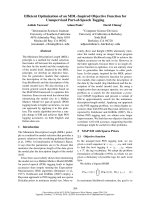
To demonstrate the use of on-the-fly application
in a cascade, we next show the effect of PRO-
DUCE when used with the cascade G◦M
A
◦M
B
,
where M
B
is in Figure 2c. Our driving al-
gorithm in this case is Algorithm 5, MAKE-
11
Note further that it allows forward application of class
wxLNT, something the embed-compose-project approach did
not allow.
12
By convention the initial nonterminal and state are listed
first in graphical depictions of WRTGs and WXTTs.
r
JJ
.JJ(x
1
, x

2
, x
3
) −→ JJ(r
DT
.x
1
, r
JJ
.x
2
, r
VB
.x
3
)
r
VB
.VB(x
1
, x
2
, x
3
) −→ VB(r
NNPS
.x
1
, r
NN

.x
3
, r
VB
.x
2
)
t.”gentle” −→ ”gentle”
(a) Rotation rules
i
VB
.NN(x
1
, x
2
) −→ NN(INS i
NN
.x
1
, i
NN
.x
2
)
i
VB
.NN(x
1
, x
2

) −→ NN(i
NN
.x
1
, i
NN
.x
2
)
i
VB
.NN(x
1
, x
2
) −→ NN(i
NN
.x
1
, i
NN
.x
2
, INS)
(b) Insertion rules
t.VB(x
1
, x
2
, x

3
) −→ X(t.x
1
, t.x
2
, t.x
3
)
t.”gentleman” −→ j1
t.”gentleman” −→ EPS
t.INS −→ j1
t.INS −→ j2
(c) Translation rules
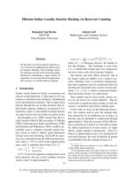
Figure 3: Example rules from transducers used
in decoding experiment. j1 and j2 are Japanese
words.
EXPLICIT, which simply generates the full ap-
plication WRTG using calls to PRODUCE. The
input to MAKE-EXPLICIT is G
2
= ({g
0
a
0
b
0
},
{σ, α}, ∅, g
0
a

0
b
0
, M
B
, G
1
).
13
MAKE-EXPLICIT
calls PRODUCE(G
2
, g
0
a
0
b
0
). PRODUCE then
seeks to cover b
0
.σ(x
1
, x
2
)
w
9
−→ σ(b
0

.x
1
, b
0
.x
2
)
with productions from G
1
, which is a stand-in for
M
A
(G)

. At line 14 of REPLACE, G
1
is im-
proved so that it has the appropriate productions.
The productions of M
A
(G)

that must be built
to form the complete M
B
(M
A
(G)

)


are shown
in Figure 2d. The complete M
B
(M
A
(G)

)

is
shown in Figure 2e. Note that because we used
this on-the-fly approach, we were able to avoid
building all the productions in M
A
(G)

; in par-
ticular we did not build g
0
a
2
w
2
·w
8
−−−−→ ρ, while a
bucket brigade approach would have built this pro-
duction. We have also designed an analogous on-
the-fly PRODUCE algorithm for backward appli-

cation on linear WTT.
We have now defined several on-the-fly and
bucket brigade algorithms, and also discussed the
possibility of embed-compose-project and offline
composition strategies to application of cascades
of tree transducers. Tables 2a and 2b summa-
rize the available methods of forward and back-
ward application of cascades for recognizability-
preserving tree transducer classes.
5 Decoding Experiments
The main purpose of this paper has been to
present novel algorithms for performing applica-
tion. However, it is important to demonstrate these
algorithms on real data. We thus demonstrate
bucket-brigade and on-the-fly backward applica-
tion on a typical NLP task cast as a cascade of
wLNT. We adapt the Japanese-to-English transla-
13
Note that G
2
is the initial stand-in for M
B
(M
A
(G)

)

,
since G

1
is the initial stand-in for M
A
(G)

.
1064
method WST wxLNT wLNT
oc
√
×
√
bb
√
×
√
otf
√ √ √
(a) Forward application
method WST wxLT wLT wxLNT wLNT
oc
√
× × ×
√
bb
√ √ √ √ √
otf
√ √ √ √ √
(b) Backward application
Table 2: Transducer types and available methods of forward and backward application of a cascade.

oc = offline composition, bb = bucket brigade, otf = on the fly.
tion model of Yamada and Knight (2001) by trans-
forming it from an English-tree-to-Japanese-string
model to an English-tree-to-Japanese-tree model.
The Japanese trees are unlabeled, meaning they
have syntactic structure but all nodes are labeled
“X”. We then cast this modified model as a cas-
cade of LNT tree transducers. Space does not per-
mit a detailed description, but some example rules
are in Figure 3. The rotation transducer R, a sam-
ple of which is in Figure 3a, has 6,453 rules, the
insertion transducer I, Figure 3b, has 8,122 rules,
and the translation transducer, T , Figure 3c, has
37,311 rules.
We add an English syntax language model L to
the cascade of transducers just described to bet-
ter simulate an actual machine translation decod-
ing task. The language model is cast as an iden-
tity WTT and thus fits naturally into the experimen-
tal framework. In our experiments we try several
different language models to demonstrate varying
performance of the application algorithms. The
most realistic language model is a PCFG. Each
rule captures the probability of a particular se-
quence of child labels given a parent label. This
model has 7,765 rules.
To demonstrate more extreme cases of the use-
fulness of the on-the-fly approach, we build a lan-
guage model that recognizes exactly the 2,087
trees in the training corpus, each with equal

weight. It has 39,455 rules. Finally, to be ultra-
specific, we include a form of the “specific” lan-
guage model just described, but only allow the
English counterpart of the particular Japanese sen-
tence being decoded in the language.
The goal in our experiments is to apply a single
tree t backward through the cascade L◦R◦I◦T ◦t
and find the 1-best path in the application WRTG.
We evaluate the speed of each approach: bucket
brigade and on-the-fly. The algorithm we use to
obtain the 1-best path is a modification of the k-
best algorithm of Pauls and Klein (2009). Our al-
gorithm finds the 1-best path in a WRTG and ad-
mits an on-the-fly approach.
The results of the experiments are shown in
Table 3. As can be seen, on-the-fly application
is generally faster than the bucket brigade, about
double the speed per sentence in the traditional
LM type method time/sentence
pcfg bucket 28s
pcfg otf 17s
exact bucket >1m
exact otf 24s
1-sent bucket 2.5s
1-sent otf .06s
Table 3: Timing results to obtain 1-best from ap-
plication through a weighted tree transducer cas-
cade, using on-the-fly vs. bucket brigade back-
ward application techniques. pcfg = model rec-
ognizes any tree licensed by a pcfg built from

observed data, exact = model recognizes each of
2,000+ trees with equal weight, 1-sent = model
recognizes exactly one tree.
experiment that uses an English PCFG language
model. The results for the other two language
models demonstrate more keenly the potential ad-
vantage that an on-the-fly approach provides—the
simultaneous incorporation of information from
all models allows application to be done more ef-
fectively than if each information source is consid-
ered in sequence. In the “exact” case, where a very
large language model that simply recognizes each
of the 2,087 trees in the training corpus is used,
the final application is so large that it overwhelms
the resources of a 4gb MacBook Pro, while the
on-the-fly approach does not suffer from this prob-
lem. The “1-sent” case is presented to demonstrate
the ripple effect caused by using on-the fly. In the
other two cases, a very large language model gen-
erally overwhelms the timing statistics, regardless
of the method being used. But a language model
that represents exactly one sentence is very small,
and thus the effects of simultaneous inference are
readily apparent—the time to retrieve the 1-best
sentence is reduced by two orders of magnitude in
this experiment.
6 Conclusion
We have presented algorithms for forward and
backward application of weighted tree trans-
ducer cascades, including on-the-fly variants, and

demonstrated the benefit of an on-the-fly approach
to application. We note that a more formal ap-
proach to application of WTTs is being developed,
1065
independent from these efforts, by F
¨
ul
¨
op et al.
(2010).
Acknowledgments
We are grateful for extensive discussions with
Andreas Maletti. We also appreciate the in-
sights and advice of David Chiang, Steve De-
Neefe, and others at ISI in the preparation of
this work. Jonathan May and Kevin Knight were
supported by NSF grants IIS-0428020 and IIS-
0904684. Heiko Vogler was supported by DFG
VO 1011/5-1.
References
Athanasios Alexandrakis and Symeon Bozapalidis.
1987. Weighted grammars and Kleene’s theorem.
Information Processing Letters, 24(1):1–4.
Brenda S. Baker. 1979. Composition of top-down and
bottom-up tree transductions. Information and Con-
trol, 41(2):186–213.
Zolt
´
an
´

Esik and Werner Kuich. 2003. Formal tree se-
ries. Journal of Automata, Languages and Combi-
natorics, 8(2):219–285.
Zolt
´
an F
¨
ul
¨
op and Heiko Vogler. 2009. Weighted tree
automata and tree transducers. In Manfred Droste,
Werner Kuich, and Heiko Vogler, editors, Handbook
of Weighted Automata, chapter 9, pages 313–404.
Springer-Verlag.
Zolt
´
an F
¨
ul
¨
op, Andreas Maletti, and Heiko Vogler.
2010. Backward and forward application of
weighted extended tree transducers. Unpublished
manuscript.
Ferenc G
´
ecseg and Magnus Steinby. 1984. Tree Au-
tomata. Akad
´
emiai Kiad

´
o, Budapest.
Liang Huang and David Chiang. 2005. Better k-best
parsing. In Harry Bunt, Robert Malouf, and Alon
Lavie, editors, Proceedings of the Ninth Interna-
tional Workshop on Parsing Technologies (IWPT),
pages 53–64, Vancouver, October. Association for
Computational Linguistics.
Werner Kuich. 1998. Formal power series over trees.
In Symeon Bozapalidis, editor, Proceedings of the
3rd International Conference on Developments in
Language Theory (DLT), pages 61–101, Thessa-
loniki, Greece. Aristotle University of Thessaloniki.
Werner Kuich. 1999. Tree transducers and formal tree
series. Acta Cybernetica, 14:135–149.
Andreas Maletti, Jonathan Graehl, Mark Hopkins, and
Kevin Knight. 2009. The power of extended top-
down tree transducers. SIAM Journal on Comput-
ing, 39(2):410–430.
Andreas Maletti. 2006. Compositions of tree se-
ries transformations. Theoretical Computer Science,
366:248–271.
Andreas Maletti. 2008. Compositions of extended top-
down tree transducers. Information and Computa-
tion, 206(9–10):1187–1196.
Andreas Maletti. 2009. Personal Communication.
Mehryar Mohri, Fernando C. N. Pereira, and Michael
Riley. 2000. The design principles of a weighted
finite-state transducer library. Theoretical Computer
Science, 231:17–32.

Mehryar Mohri. 1997. Finite-state transducers in lan-
guage and speech processing. Computational Lin-
guistics, 23(2):269–312.
Mehryar Mohri. 2009. Weighted automata algo-
rithms. In Manfred Droste, Werner Kuich, and
Heiko Vogler, editors, Handbook of Weighted Au-
tomata, chapter 6, pages 213–254. Springer-Verlag.
Adam Pauls and Dan Klein. 2009. K-best A* parsing.
In Keh-Yih Su, Jian Su, Janyce Wiebe, and Haizhou
Li, editors, Proceedings of the Joint Conference of
the 47th Annual Meeting of the ACL and the 4th In-
ternational Joint Conference on Natural Language
Processing of the AFNLP, pages 958–966, Suntec,
Singapore, August. Association for Computational
Linguistics.
Fernando Pereira and Michael Riley. 1997. Speech
recognition by composition of weighted finite au-
tomata. In Emmanuel Roche and Yves Schabes, ed-
itors, Finite-State Language Processing, chapter 15,
pages 431–453. MIT Press, Cambridge, MA.
William A. Woods. 1980. Cascaded ATN gram-
mars. American Journal of Computational Linguis-
tics, 6(1):1–12.
Kenji Yamada and Kevin Knight. 2001. A syntax-
based statistical translation model. In Proceedings
of 39th Annual Meeting of the Association for Com-
putational Linguistics, pages 523–530, Toulouse,
France, July. Association for Computational Lin-
guistics.
1066