Image estimation by example geophysical sounding j claerbout

IMAGE ESTIMATION BY EXAMPLE:
Geophysical soundings image construction
Multidimensional autoregression
Jon F. Claerbout
Cecil and Ida Green Professor of Geophysics
Stanford University
with
Sergey Fomel
Stanford University
c
 February 28, 2006

dedicated to the memory
of
Johannes “Jos” Claerbout
1974-1999
“What do we have to look forward to today?
There are a lot of things we have to look forward to today.”
/>
Contents
1 Basic operators and adjoints 1
1.1 FAMILIAR OPERATORS . . . . . . . . . . . . . . . . . . . . . . . . . . . 5
1.2 ADJOINT DEFINED: DOT-PRODUCT TEST . . . . . . . . . . . . . . . . 27
2 Model fitting by least squares 33
2.1 HOW TO DIVIDE NOISY SIGNALS . . . . . . . . . . . . . . . . . . . . . 33
2.2 MULTIVARIATE LEAST SQUARES . . . . . . . . . . . . . . . . . . . . . 39
2.3 KRYLOV SUBSPACE ITERATIVE METHODS . . . . . . . . . . . . . . . 45
2.4 INVERSE NMO STACK . . . . . . . . . . . . . . . . . . . . . . . . . . . . 56
2.5 VESUVIUS PHASE UNWRAPPING . . . . . . . . . . . . . . . . . . . . . 57
2.6 THE WORLD OF CONJUGATE GRADIENTS . . . . . . . . . . . . . . . . 66
2.7 REFERENCES . . . . . . . . . . . . . . . . . . . . . . . . . . . . . . . . . 72

3 Empty bins and inverse interpolation 73
3.1 MISSING DATA IN ONE DIMENSION . . . . . . . . . . . . . . . . . . . . 74
3.2 WELLS NOT MATCHING THE SEISMIC MAP . . . . . . . . . . . . . . . 82
3.3 SEARCHING THE SEA OF GALILEE . . . . . . . . . . . . . . . . . . . . 87
3.4 INVERSE LINEAR INTERPOLATION . . . . . . . . . . . . . . . . . . . . 90
3.5 PREJUDICE, BULLHEADEDNESS, AND CROSS VALIDATION . . . . . 94
4 The helical coordinate 97
4.1 FILTERING ON A HELIX . . . . . . . . . . . . . . . . . . . . . . . . . . . 97
4.2 FINITE DIFFERENCES ON A HELIX . . . . . . . . . . . . . . . . . . . . 107
CONTENTS
4.3 CAUSALITY AND SPECTAL FACTORIZATION . . . . . . . . . . . . . . 111
4.4 WILSON-BURG SPECTRAL FACTORIZATION . . . . . . . . . . . . . . 116
4.5 HELIX LOW-CUT FILTER . . . . . . . . . . . . . . . . . . . . . . . . . . 120
4.6 THE MULTIDIMENSIONAL HELIX . . . . . . . . . . . . . . . . . . . . . 123
4.7 SUBSCRIPTING A MULTIDIMENSIONAL HELIX . . . . . . . . . . . . . 124
5 Preconditioning 131
5.1 PRECONDITIONED DATA FITTING . . . . . . . . . . . . . . . . . . . . . 131
5.2 PRECONDITIONING THE REGULARIZATION . . . . . . . . . . . . . . 132
5.3 OPPORTUNITIES FOR SMART DIRECTIONS . . . . . . . . . . . . . . . 137
5.4 NULL SPACE AND INTERVAL VELOCITY . . . . . . . . . . . . . . . . . 138
5.5 INVERSE LINEAR INTERPOLATION . . . . . . . . . . . . . . . . . . . . 143
5.6 EMPTY BINS AND PRECONDITIONING . . . . . . . . . . . . . . . . . . 146
5.7 THEORY OF UNDERDETERMINED LEAST-SQUARES . . . . . . . . . . 150
5.8 SCALING THE ADJOINT . . . . . . . . . . . . . . . . . . . . . . . . . . . 151
5.9 A FORMAL DEFINITION FOR ADJOINTS . . . . . . . . . . . . . . . . . 153
6 Multidimensional autoregression 155
6.1 SOURCE WAVEFORM, MULTIPLE REFLECTIONS . . . . . . . . . . . . 156
6.2 TIME-SERIES AUTOREGRESSION . . . . . . . . . . . . . . . . . . . . . 157
6.3 PREDICTION-ERROR FILTER OUTPUT IS WHITE . . . . . . . . . . . . 159
6.4 PEF ESTIMATION WITH MISSING DATA . . . . . . . . . . . . . . . . . 174

6.5 TWO-STAGE LINEAR LEAST SQUARES . . . . . . . . . . . . . . . . . . 178
6.6 BOTH MISSING DATA AND UNKNOWN FILTER . . . . . . . . . . . . . 186
6.7 LEVELED INVERSE INTERPOLATION . . . . . . . . . . . . . . . . . . . 190
6.8 MULTIVARIATE SPECTRUM . . . . . . . . . . . . . . . . . . . . . . . . 194
7 Noisy data 199
7.1 MEANS, MEDIANS, PERCENTILES AND MODES . . . . . . . . . . . . 199
7.2 NOISE BURSTS . . . . . . . . . . . . . . . . . . . . . . . . . . . . . . . . 208
7.3 MEDIAN BINNING . . . . . . . . . . . . . . . . . . . . . . . . . . . . . . 209
CONTENTS
7.4 ROW NORMALIZED PEF . . . . . . . . . . . . . . . . . . . . . . . . . . . 210
7.5 DEBURST . . . . . . . . . . . . . . . . . . . . . . . . . . . . . . . . . . . 211
7.6 TWO 1-D PEFS VERSUS ONE 2-D PEF . . . . . . . . . . . . . . . . . . . 213
7.7 ALTITUDE OF SEA SURFACE NEAR MADAGASCAR . . . . . . . . . . 215
7.8 ELIMINATING NOISE AND SHIP TRACKS IN GALILEE . . . . . . . . . 220
8 Spatial aliasing and scale invariance 233
8.1 INTERPOLATION BEYOND ALIASING . . . . . . . . . . . . . . . . . . . 233
8.2 MULTISCALE, SELF-SIMILAR FITTING . . . . . . . . . . . . . . . . . . 236
8.3 References . . . . . . . . . . . . . . . . . . . . . . . . . . . . . . . . . . . . 242
9 Nonstationarity: patching 243
9.1 PATCHING TECHNOLOGY . . . . . . . . . . . . . . . . . . . . . . . . . . 244
9.2 STEEP-DIP DECON . . . . . . . . . . . . . . . . . . . . . . . . . . . . . . 251
9.3 INVERSION AND NOISE REMOVAL . . . . . . . . . . . . . . . . . . . . 257
9.4 SIGNAL-NOISE DECOMPOSITION BY DIP . . . . . . . . . . . . . . . . 257
9.5 SPACE-VARIABLE DECONVOLUTION . . . . . . . . . . . . . . . . . . . 264
10 Plane waves in three dimensions 271
10.1 THE LEVELER: A VOLUME OR TWO PLANES? . . . . . . . . . . . . . 271
10.2 WAVE INTERFERENCE AND TRACE SCALING . . . . . . . . . . . . . . 275
10.3 LOCAL MONOPLANE ANNIHILATOR . . . . . . . . . . . . . . . . . . . 276
10.4 GRADIENT ALONG THE BEDDING PLANE . . . . . . . . . . . . . . . . 280
10.5 3-D SPECTRAL FACTORIZATION . . . . . . . . . . . . . . . . . . . . . . 283

11 Some research examples 285
11.1 GULF OF MEXICO CUBE . . . . . . . . . . . . . . . . . . . . . . . . . . 285
12 SOFTWARE SUPPORT 287
12.1 SERGEY’S MAIN PROGRAM DOCS . . . . . . . . . . . . . . . . . . . . 290
12.2 References . . . . . . . . . . . . . . . . . . . . . . . . . . . . . . . . . . . . 300
CONTENTS
13 Entrance examination 301
Index 303
Preface
The difference between theory and practice is smaller in theory than it is in
practice. –folklore
We make discoveries about reality by examining the discrepancy between theory and practice.
There is a well-developed theory about the difference between theory and practice, and it is
called “geophysical inverse theory”. In this book we investigate the practice of the difference
between theory and practice. As the folklore tells us, there is a big difference. There are
already many books on the theory, and often as not, they end in only one or a few applications
in the author’s specialty. In this book on practice, we examine data and results from many
diverse applications. I have adopted the discipline of suppressing theoretical curiosities until I
find data that requires it (except for a few concepts at chapter ends).
Books on geophysical inverse theory tend to address theoretical topics that are little used
in practice. Foremost is probability theory. In practice, probabilities are neither observed nor
derived from observations. For more than a handful of variables, it would not be practical
to display joint probabilities, even if we had them. If you are data poor, you might turn to
probabilities. If you are data rich, you have far too many more rewarding things to do. When
you estimate a few values, you ask about their standard deviations. When you have an image
making machine, you turn the knobs and make new images (and invent new knobs). Another
theory not needed here is singular-value decomposition.
In writing a book on the “practice of the difference between theory and practice" there is
no worry to be bogged down in the details of diverse specializations because the geophysi-
cal world has many interesting data sets that are easily analyzed with elementary physics and

simple geometry. (My specialization, reflection seismic imaging, has a great many less easily
explained applications too.) We find here many applications that have a great deal in com-
mon with one another, and that commonality is not a part of common inverse theory. Many
applications draw our attention to the importance of two weighting functions (one required
for data space and the other for model space). Solutions depend strongly on these weighting
functions (eigenvalues do too!). Where do these functions come from, from what rationale or
estimation procedure? We’ll see many examples here, and find that these functions are not
merely weights but filters. Even deeper, they are generally a combination of weights and fil-
ters. We do some tricky bookkeeping and bootstrapping when we filter the multidimensional
neighborhood of missing and/or suspicious data.
Are you aged 23? If so, this book is designed for you. Life has its discontinuities: when
i
ii
CONTENTS
you enter school at age 5, when you leave university, when you marry, when you retire. The
discontinuity at age 23, mid graduate school, is when the world loses interest in your potential
to learn. Instead the world wants to know what you are accomplishing right now! This book
is about how to make images. It is theory and programs that you can use right now.
This book is not devoid of theory and abstraction. Indeed it makes an important new
contribution to the theory (and practice) of data analysis: multidimensional autoregression via
the helical coordinate system.
The biggest chore in the study of “the practice of the difference between theory and prac-
tice" is that we must look at algorithms. Some of them are short and sweet, but other important
algorithms are complicated and ugly in any language. This book can be printed without the
computer programs and their surrounding paragraphs, or you can read it without them. I
suggest, however, you take a few moments to try to read each program. If you can write in
any computer language, you should be able to read these programs well enough to grasp the
concept of each, to understand what goes in and what should come out. I have chosen the
computer language (more on this later) that I believe is best suited for our journey through the
“elementary” examples in geophysical image estimation.

Besides the tutorial value of the programs, if you can read them, you will know exactly
how the many interesting illustrations in this book were computed so you will be well equipped
to move forward in your own direction.
THANKS
2006 is my fourteenth year of working on this book and much of it comes from earlier work
and the experience of four previous books. In this book, as in my previous books, I owe a
great deal to the many students at the Stanford Exploration Project. I would like to mention
some with particularly notable contributions (in approximate historical order).
The concept of this book began along with the PhD thesis of Jeff Thorson. Before that,
we imagers thought of our field as "an hoc collection of good ideas" instead of as "adjoints of
forward problems". Bill Harlan understood most of the preconditioning issues long before I
did. All of us have a longstanding debt to Rick Ottolini who built a cube movie program long
before anyone else in the industry had such a blessing.
My first book was built with a typewriter and ancient technologies. In early days each
illustration would be prepared without reusing packaged code. In assembling my second book
I found I needed to develop common threads and code them only once and make this code sys-
tematic and if not idiot proof, then “idiot resistant”. My early attempts to introduce “seplib”
were not widely welcomed until Stew Levin rebuilt everything making it much more robust.
My second book was typed in the troff text language. I am indebted to Kamal Al-Yahya who
not only converted that book to L
A
T
E
X, but who wrote a general-purpose conversion program
that became used internationally.
Early days were a total chaos of plot languages. I and all the others at SEP are deeply
CONTENTS
iii
indebted to Joe Dellinger who starting from work of Dave Hale, produced our internal plot
language “vplot” which gave us reproducibiliy and continuity over decades. Now, for exam-

ple, our plots seamlessly may be directed to postscript (and PDF), Xwindow, or the web. My
second book required that illustrations be literally taped onto the sheet containing the words.
All of us benefitted immensely from the work of Steve Cole who converted Joe’s vplot lan-
guage to postscript which was automatically integrated with the text.
When I began my third book I was adapting liberally from earlier work. I began to realize
the importance of being able to reproduce any earlier calculation and began building rules and
file-naming conventions for “reproducible research”. This would have been impossible were
it not for Dave Nichols who introduced cake, a variant of the UNIX software building pro-
gram make. Martin Karrenbach continued the construction of our invention of “reproducible
research” and extended it to producing reproducible research reports on CD-ROM, an idea
well ahead of its time. Some projects were fantastic for their time but had the misfortune of
not being widely adopted, ultimately becoming unsupportable. In this catagory was Dave and
Martin’s implementation xtex, a magnificent way of embedding reproducible research in an
electronic textbook. When cake suffered the same fate as xtex, Matthias Schwab saved us
from mainstream isolation by bringing our build procedures into the popular GNU world.
Coming to the present textbook I mention Bob Clapp. He made numerous contributions.
When Fortran77 was replaced by Fortran90, he rewrote Ratfor. For many years I (and many
of us) depended on Ratfor as our interface to Fortran and as a way of presenting uncluttered
code. Bob rewrote Ratfor from scratch merging it with other SEP-specific software tools (Sat)
making Ratfor90. Bob prepared the interval-velocity examples in this book. Bob also devel-
oped most of the “geostat” ideas and examples in this book. Morgan Brown introduced the
texture examples that we find so charming. Paul Sava totally revised the book’s presentation
of least-squares solvers making them more palatable to students and making more honest our
claim that in each case the results you see were produced by the code you see.
One name needs to be singled out. Sergey Fomel converted all the examples in this book
from my original Fortran 77 to a much needed modern style of Fortran 90. After I discovered
the helix idea and its wide-ranging utility, he adapted all the relevant examples in this book
to use it. If you read Fomel’s programs, you can learn effective application of that 1990’s
revolution in coding style known as “object orientation.”
This electronic book, “Geophysical Exploration by Example,” is free software; you can redistribute it

and/or modify it under the terms of the GNU General Public License as published by the Free Software
Foundation; either version 2 of the License, or (at your option) any later version. This book is distributed
in the hope that it will be useful, but WITHOUT ANY WARRANTY; without even the implied warranty
of MERCHANTABILITY or FITNESS FOR A PARTICULAR PURPOSE. See the GNU General Public
License for more details. You should have received a copy of the GNU General Public License along with
this program; if not, write to the Free Software Foundation, Inc., 675 Massachusetts Ave., Cambridge, MA
02139, USA.
c
Jon Claerbout
February 28, 2006
iv
CONTENTS
Overview
This book is about the estimation and construction of geophysical images. Geophysical images
are used to visualize petroleum and mineral resource prospects, subsurface water, contaminent
transport (environmental pollution), archeology, lost treasure, even graves.
Here we follow physical measurements from a wide variety of geophysical sounding de-
vices to a geophysical image, a 1-, 2-, or 3-dimensional Cartesian mesh that is easily trans-
formed to a graph, map image, or computer movie. A later more human, application-specific
stage (not addressed here) interprets and annotates the images; that stage places the “×” where
you will drill, dig, dive, or merely dream.
Image estimation is a subset of “geophysical inverse theory,” itself a kind of “theory of
how to find everything.” In contrast to “everything,” images have an organized structure (co-
variance) that makes their estimation more concrete and visual, and leads to the appealing
results we find here.
Geophysical sounding data used in this book comes from acoustics, radar, and seismology.
Sounders are operated along tracks on the earth surface (or tracks in the ocean, air, or space). A
basic goal of data processing is an image that shows the earth itself, not an image of our data-
acquisition tracks. We want to hide our data acquisition footprint. Increasingly, geophysicists
are being asked to measure changes in the earth by comparing old surveys to new ones. Then

we are involved with both the old survey tracks and new ones, as well as technological changes
between old sounders and new ones.
To enable this book to move rapidly along from one application to another, we avoid appli-
cations where the transform from model to data is mathematically complicated, but we include
the central techniques of constructing the adjoint of any such complicated transformation. By
setting aside application-specific complications, we soon uncover and deal with universal dif-
ficulties such as: (1) irregular geometry of recording, (2) locations where no recording took
place and, (3) locations where crossing tracks made inconsistant measurements because of
noise. Noise itself comes in three flavors: (1) drift (zero to low frequency), (2) white or steady
and stationary broad band, and (3) bursty, i.e., large and erratic.
Missing data and inconsistant data are two humble, though universal problems. Because
they are universal problems, science and engineering have produced a cornucopia of ideas
ranging from mathematics (Hilbert adjoint) to statistics (inverse covariance) to conceptual
(stationary, scale-invariant) to numerical analysis (conjugate direction, preconditioner) to com-
puter science (object oriented) to simple common sense. Our guide through this maze of op-
v
vi
CONTENTS
portunities and digressions is the test of what works on real data, what will make a better
image. My logic for organizing the book is simply this: Easy results first. Harder results later.
Undemonstrated ideas last or not at all, and latter parts of chapters can be skimmed.
Examples here are mostly nonseismological although my closest colleagues and I mostly
make images from seismological data. The construction of 3-D subsurface landform images
from seismological data is an aggressive industry, a complex and competitive place where it is
not easy to build yourself a niche. I wrote this book because I found that beginning researchers
were often caught between high expectations and concrete realities. They invent a new process
to build a novel image but they have many frustrations: (1) lack of computer power, (2) data-
acquisition limitations (gaps, tracks, noises), or (3) they see chaotic noise and have difficulty
discerning whether the noise represents chaos in the earth, chaos in the data acquisition, chaos
in the numerical analysis, or unrealistic expectations.

People need more practice with easier problems like the ones found in this book, which
are mostly simple 2-D landforms derived from 2-D data. Such concrete estimation problems
are solved quickly, and their visual results provide experience in recognizing weaknesses,
reformulating, and moving forward again. Many small steps reach a mountain top.
Scaling up to big problems
Although most the examples in this book are presented as toys, where results are obtained
in a few minutes on a home computer, we have serious industrial-scale jobs always in the
backs of our minds. This forces us to avoid representing operators as matrices. Instead we
represent operators as a pair of subroutines, one to apply the operator and one to apply the
adjoint (transpose matrix). (This will be more clear when you reach the middle of chapter 2.)
By taking a function-pair approach to operators instead of a matrix approach, this book
becomes a guide to practical work on realistic-sized data sets. By realistic, I mean as large
and larger than those here; i.e., data ranging over two or more dimensions, and the data space
and model space sizes being larger than about 10
5
elements, about a 300 ×300 image. Even
for these, the world’s biggest computer would be required to hold in random access memory
the 10
5
×10
5
matrix linking data and image. Mathematica, Matlab, kriging, etc, are nice tools
but
1
it was no surprise when a curious student tried to apply one to an example from this
book and discovered that he needed to abandon 99.6% of the data to make it work. Matrix
methods are limited not only by the size of the matrices but also by the fact that the cost to
multiply or invert is proportional to the third power of the size. For simple experimental work,
this limits the matrix approach to data and images of about 4000 elements, a low-resolution
64 ×64 image.

1
I do not mean to imply that these tools cannot be used in the function-pair style of this book, only that
beginners tend to use a matrix approach.
CONTENTS
vii
0.0.1 Computer Languages
One feature of this book is that it teaches how to use "object programming". Older languages
like Fortran 77, Matlab, C, and Visual Basic, are not object-oriented languages. The introduc-
tion of object-oriented languages like C++, Java, and Fortran 90 a couple decades back greatly
simplified many application programs. An earlier version of this book used Fortran 77. I had
the regrettable experience that issues of Geophysics were constantly being mixed in the same
program as issues of Mathematics. This is easily avoided in object-based languages. For ease
of debugging and for ease of understanding, we want to keep the mathematical technicalities
away from the geophysical technicalities. This is called "information hiding".
In the older languages it is easy for a geophysical application program to call a mathe-
matical subroutine. That is new code calling old code. The applications we encounter in this
book require the opposite, old optimization code written by someone with a mathematical hat
calling linear operator code written by someone with a geophysical hat. The older code must
handle objects of considerable complexity only now being built by the newer code. It must
handle them as objects without knowing what is inside them. Linear operators are concep-
tually just matrix multiply (and its transpose), but concretely they are not simply matrices.
While a matrix is simply a two-dimensional array, a sparse matrix may be specified by many
components.
The newer languages allow information hiding but a price paid, from my view as a text-
book author, is that the codes are longer, hence make the book uglier. Many more initial lines
of code are taken up by definitions and declarations making my simple textbook codes about
twice as lengthy as in the older languages. This is not a disadvantage for the reader who can
rapidly skim over what soon become familiar definitions.
Of the three object-based languages available, I chose Fortran because, as its name implies,
it looks most like mathematics. Fortran has excellent primary support for multidimensional

cartesian arrays and complex numbers, unlike Java and C++. Fortran, while looked down upon
by the computer science community, is the language of choice among physicists, mechanical
engineers, and numerical analysts. While our work is certainly complex, in computer science
their complexity is more diverse.
The Loptran computer dialect
Along with theory, illustrations, and discussion, I display the programs that created the illus-
trations. To reduce verbosity in these programs, my colleagues and I have invented a little
language called Loptran that is readily translated to Fortran 90. I believe readers without For-
tran experience will comfortably be able to read Loptran, but they should consult a Fortran
book if they plan to write it. Loptran is not a new language compiler but a simple text pro-
cessor that expands concise scientific language into the more verbose expressions required by
Fortran 90.
The name Loptran denotes Linear OPerator TRANslator. The limitation of Fortran 77
viii
CONTENTS
overcome by Fortran 90 and Loptran is that we can now isolate natural science application
code from computer science least-squares fitting code, thus enabling practitioners in both dis-
ciplines to have more ready access to one anothers intellectual product.
Fortran is the original language shared by scientific computer applications. The people
who invented C and UNIX also made Fortran more readable by their invention of Ratfor
2
.
Sergey Fomel, Bob Clapp, and I have taken the good ideas from original Ratfor and merged
them with concepts of linear operators to make Loptran, a language with much the syntax of
modern languages like C++ and Java. Loptran is a small and simple adaptation of well-tested
languages, and translates to one. Loptran is, however, new in 1998 and is not yet widely used.
To help make everyone comfortable with Loptran as a generic algorithmic language, this
book avoids special features of Fortran. This should make it easier for some of you to translate
to your favorite language, such as Matlab, Java, C, or C++.
We provide the Loptran translator free. It is written in another free language, PERL, and

therefore should be available free to nearly everyone. If you prefer not to use Ratfor90 and
Loptran, you can find on the WWW
3
the Fortran 90 version of the programs in this book.
Reproducibility
Earlier versions of this series of electronic books were distributed on CD-ROM. The idea is
that each computed figure in the book has in its caption a menu allowing the reader to burn
and rebuild the figures (and movies). This idea persists in the Web book versions (as do the
movies) except that now the more difficult task of installing the basic Stanford libraries is the
obligation of the reader. Hopefully, as computers mature, this obstacle will be less formidable.
Anyway, these libraries are also offered free on our web site.
Preview for inverse theorists
People who are already familiar with “geophysical inverse theory” may wonder what new
they can gain from a book focused on “estimation of images.” Given a matrix relation d = Fm
between model m and data d, common sense suggests that practitioners should find m in
order to minimize the length ||r|| of the residual r =Fm−d. A theory of Gauss suggests that
a better (minimum variance, unbiased) estimate results from minimizing the quadratic form
r

σ
−1
rr
r, where σ
rr
is the noise covariance matrix. I have never seen an application in which
the noise covariance matrix was given, but practitioners often find ways to estimate it: they
regard various sums as ensemble averages.
Additional features of inverse theory are exhibited by the partitioned matrix
d =


d
incons
d
consis

=

0 0
B 0

m
fit
m
null

= Fm (1)
2
/>3
/>CONTENTS
ix
which shows that a portion d
incons
of the data should vanish for any model m, so an observed
nonvanishing d
incons
is inconsistent with any theoretical model m. Likewise the m
null
part of
the model space makes no contribution to the data space, so it seems not knowable from the
data.

Simple inverse theory suggests we should minimize ||m||which amounts to setting the null
space to zero. Baysian inverse theory says we should use the model covariance matrix σ
mm
and minimize m

σ
−1
mm
m for a better answer although it would include some nonzero portion of
the null space. Never have I seen an application in which the model-covariance matrix was a
given prior. Specifying or estimating it is a puzzle for experimentalists. For example, when a
model space m is a signal (having components that are a function of time) or, a stratified earth
model (with components that are function of depth z) we might supplement the fitting goal
0 ≈ r = Fm −d with a “minimum wiggliness” goal like dm(z)/dz ≈ 0. Neither the model
covariance matrix nor the null space m
null
seems learnable from the data and equation (0.1).
In fact, both the null space and the model covariance matrix can be estimated from the
data and that is one of the novelties of this book. To convince you it is possible (without
launching into the main body of the book), I offer a simple example of an operator and data
set from which your human intuition will immediately tell you what you want for the whole
model space, including the null space. Consider the data to be a sinusoidal function of time
(or depth) and take B = I so that the operator F is a delay operator with truncation of the
signal shifted off the end of the space. Solving for m
fit
, the findable part of the model, you
get a back-shifted sinusoid. Your human intuition, not any mathematics here, tells you that the
truncated part of the model, m
null
, should be a logical continuation of the sinusoid m

fit
at the
same frequency. It should not have a different frequency nor become a square wave nor be a
sinusoid abruptly truncated to zero m
null
= 0.
Prior knowledge exploited in this book is that unknowns are functions of time and space
(so the covariance matrix has known structure). This structure gives them predictability.
Predictable functions in 1-D are tides, in 2-D are lines on images (linements), in 3-D are sedi-
mentary layers, and in 4-D are wavefronts. The tool we need to best handle this predictability
is the multidimensional “prediction-error filter” (PEF), a central theme of this book.
x
CONTENTS
Chapter 1
Basic operators and adjoints
A great many of the calculations we do in science and engineering are really matrix mul-
tiplication in disguise. The first goal of this chapter is to unmask the disguise by showing
many examples. Second, we see how the adjoint operator (matrix transpose) back projects
information from data to the underlying model.
Geophysical modeling calculations generally use linear operators that predict data from
models. Our usual task is to find the inverse of these calculations; i.e., to find models (or make
images) from the data. Logically, the adjoint is the first step and a part of all subsequent steps
in this inversion process. Surprisingly, in practice the adjoint sometimes does a better job than
the inverse! This is because the adjoint operator tolerates imperfections in the data and does
not demand that the data provide full information.
Using the methods of this chapter, you will find that once you grasp the relationship be-
tween operators in general and their adjoints, you can obtain the adjoint just as soon as you
have learned how to code the modeling operator.
If you will permit me a poet’s license with words, I will offer you the following table of
operators and their adjoints:

matrix multiply conjugate-transpose matrix multiply
convolve crosscorrelate
truncate zero pad
replicate, scatter, spray sum or stack
spray into neighborhoods sum within bins
derivative (slope) negative derivative
causal integration anticausal integration
add functions do integrals
assignment statements added terms
plane-wave superposition slant stack / beam form
superpose curves sum along a curve
stretch squeeze
scalar field gradient negative of vector field divergence
1
2
CHAPTER 1. BASIC OPERATORS AND ADJOINTS
upward continue downward continue
diffraction modeling imaging by migration
hyperbola modeling CDP stacking
ray tracing tomography
The left column above is often called “modeling,” and the adjoint operators on the right
are often used in “data processing.”
When the adjoint operator is not an adequate approximation to the inverse, then you apply
the techniques of fitting and optimization explained in Chapter 2. These techniques require
iterative use of the modeling operator and its adjoint.
The adjoint operator is sometimes called the “back projection” operator because infor-
mation propagated in one direction (earth to data) is projected backward (data to earth model).
Using complex-valued operators, the transpose and complex conjugate go together; and in
Fourier analysis, taking the complex conjugate of exp(iωt) reverses the sense of time. With
more poetic license, I say that adjoint operators undo the time and phase shifts of modeling

operators. The inverse operator does this too, but it also divides out the color. For example,
when linear interpolation is done, then high frequencies are smoothed out, so inverse inter-
polation must restore them. You can imagine the possibilities for noise amplification. That
is why adjoints are safer than inverses. But nature determines in each application what is the
best operator to use, and whether to stop after the adjoint, to go the whole way to the inverse,
or to stop partway.
The operators and adjoints above transform vectors to other vectors. They also transform
data planes to model planes, volumes, etc. A mathematical operator transforms an “abstract
vector” which might be packed full of volumes of information like television signals (time
series) can pack together a movie, a sequence of frames. We can always think of the operator
as being a matrix but the matrix can be truly huge (and nearly empty). When the vectors
transformed by the matrices are large like geophysical data set sizes then the matrix sizes
are “large squared,” far too big for computers. Thus although we can always think of an
operator as a matrix, in practice, we handle an operator differently. Each practical application
requires the practitioner to prepare two computer programs. One performs the matrix multiply
y = Ax and another multiplys by the transpose
˜
x = A

y (without ever having the matrix itself
in memory). It is always easy to transpose a matrix. It is less easy to take a computer program
that does y =Ax and convert it to another to do
˜
x =A

y. In this chapter are many examples of
increasing complexity. At the end of the chapter we will see a test for any program pair to see
whether the operators A and A

are mutually adjoint as they should be. Doing the job correctly

(coding adjoints without making approximations) will reward us later when we tackle model
and image estimation problems.
3
1.0.1 Programming linear operators
The operation y
i
=

j
b
ij
x
j
is the multiplication of a matrix B by a vector x. The adjoint
operation is ˜x
j
=

i
b
ij
y
i
. The operation adjoint to multiplication by a matrix is multiplication
by the transposed matrix (unless the matrix has complex elements, in which case we need the
complex-conjugated transpose). The following pseudocode does matrix multiplication y=Bx
and multiplication by the transpose
˜
x = B


y:
if adjoint
then erase x
if operator itself
then erase y
do iy = 1, ny {
do ix = 1, nx {
if adjoint
x(ix) = x(ix) + b(iy,ix) × y(iy)
if operator itself
y(iy) = y(iy) + b(iy,ix) × x(ix)
}}
Notice that the “bottom line” in the program is that x and y are simply interchanged. The
above example is a prototype of many to follow, so observe carefully the similarities and
differences between the adjoint and the operator itself.
Next we restate the matrix-multiply pseudo code in real code, in a language called Lop-
tran
1
, a language designed for exposition and research in model fitting and optimization in
physical sciences. The module matmult for matrix multiply and its adjoint exhibits the style
that we will use repeatedly. At last count there were 53 such routines (operator with adjoint)
in this book alone.
module matmult { # matrix multiply and its adjoint
real, dimension (:,:), pointer :: bb
#% _init( bb)
#% _lop( x, y)
integer ix, iy
do ix= 1, size(x) {
do iy= 1, size(y) {
if( adj)

x(ix) = x(ix) + bb(iy,ix) * y(iy)
else
y(iy) = y(iy) + bb(iy,ix) * x(ix)
}}
}
1
The programming language, Loptran, is based on a dialect of Fortran called Ratfor. For more details, see
Appendix A.
4
CHAPTER 1. BASIC OPERATORS AND ADJOINTS
Notice that the module matmult does not explicitly erase its output before it begins, as does
the psuedo code. That is because Loptran will always erase for you the space required for the
operator’s output. Loptran also defines a logical variable adj for you to distinguish your com-
putation of the adjoint x=x+B’*y from the forward operation y=y+B*x. In computerese, the two
lines beginning #% are macro expansions that take compact bits of information which expand
into the verbose boilerplate that Fortran requires. Loptran is Fortran with these macro expan-
sions. You can always see how they expand by looking at />What is new in Fortran 90, and will be a big help to us, is that instead of a subroutine
with a single entry, we now have a module with two entries, one named _init for the physical
scientist who defines the physical problem by defining the matrix, and another named _lop for
the least-squares problem solver, the computer scientist who will not be interested in how we
specify B, but who will be iteratively computing Bx and B

y to optimize the model fitting. The
lines beginning with #% are expanded by Loptran into more verbose and distracting Fortran 90
code. The second line in the module matmult, however, is pure Fortran syntax saying that bb
is a pointer to a real-valued matrix.
To use matmult, two calls must be made, the first one
call matmult_init( bb)
is done by the physical scientist after he or she has prepared the matrix. Most later calls will
be done by numerical analysts in solving code like in Chapter 2. These calls look like

stat = matmult_lop( adj, add, x, y)
where adj is the logical variable saying whether we desire the adjoint or the operator itself,
and where add is a logical variable saying whether we want to accumulate like y ← y +Bx
or whether we want to erase first and thus do y ← Bx. The return value stat is an integer
parameter, mostly useless (unless you want to use it for error codes).
Operator initialization often allocates memory. To release this memory, you can call
matmult_close() although in this case nothing really happens.
We split operators into two independent processes, the first is used for geophysical set up
while the second is invoked by mathematical library code (introduced in the next chapter) to
find the model that best fits the data. Here is why we do so. It is important that the math code
contain nothing about the geophysical particulars. This enables us to use the same math code
on many different geophysical problems. This concept of “information hiding” arrived late
in human understanding of what is desireable in a computer language. This feature alone is
valuable enough to warrant upgrading from Fortran 77 to Fortran 90, and likewise from C to
C++. Subroutines and functions are the way that new programs use old ones. Object modules
are the way that old programs (math solvers) are able to use new ones (geophysical operators).
1.1. FAMILIAR OPERATORS
5
1.1 FAMILIAR OPERATORS
The simplest and most fundamental linear operators arise when a matrix operator reduces to a
simple row or a column.
A row is a summation operation.
A column is an impulse response.
If the inner loop of a matrix multiply ranges within a
row, the operator is called sum or pull.
column, the operator is called spray or push.
A basic aspect of adjointness is that the adjoint of a row matrix operator is a column matrix
operator. For example, the row operator [a,b]
y = [ a b ]


x
1
x
2

= ax
1
+bx
2
(1.1)
has an adjoint that is two assignments:

ˆx
1
ˆx
2

=

a
b

y (1.2)
The adjoint of a sum of N terms is a collection of N assignments.
1.1.1 Adjoint derivative
In numerical analysis we represent the derivative a time function by a finite difference. We do
this by subtracting each two neighboring time points and then dividing by the sample interval
t. This amounts to convolution with the filter (1,−1)/t. Omitting the t we express this
concept as:









y
1
y
2
y
3
y
4
y
5
y
6








=









−1 1 . . . .
. −1 1 . . .
. . −1 1 . .
. . . −1 1 .
. . . . −1 1
. . . . . 0
















x
1

x
2
x
3
x
4
x
5
x
6








(1.3)
The filter impulse response is seen in any column in the middle of the matrix, namely
(1, −1). In the transposed matrix, the filter-impulse response is time-reversed to (−1,1). So,
mathematically, we can say that the adjoint of the time derivative operation is the negative
6
CHAPTER 1. BASIC OPERATORS AND ADJOINTS
time derivative. This corresponds also to the fact that the complex conjugate of −iω is iω. We
can also speak of the adjoint of the boundary conditions: we might say that the adjoint of “no
boundary condition” is a “specified value” boundary condition. The last row in equation (1.3)
is optional. It may seem unnatural to append a null row, but it can be a small convenience
(when plotting) to have the input and output be the same size.
Equation (1.3) is implemented by the code in module igrad1 which does the operator itself

(the forward operator) and its adjoint.
module igrad1 { # gradient in one dimension
#% _lop( xx, yy)
integer i
do i= 1, size(xx)-1 {
if( adj) {
xx(i+1) = xx(i+1) + yy(i) # resembles equation (1.2)
xx(i ) = xx(i ) - yy(i)
}
else
yy(i) = yy(i) + xx(i+1) - xx(i) # resembles equation (1.1)
}
}
The adjoint code may seem strange. It might seem more natural to code the adjoint to be the
negative of the operator itself and then make the special adjustments for the boundaries. The
code given, however, is correct and requires no adjustments at the ends. To see why, notice
for each value of i, the operator itself handles one row of equation (1.3) while for each i the
adjoint handles one column. That’s why coding the adjoint in this way does not require any
special work on the ends. The present method of coding reminds us that the adjoint of a sum
of N terms is a collection of N assignments.
The Ratfor90 dialect of Fortran allows us to write the inner code of the igrad1 module
more simply and symmetrically using the syntax of C, C++, and Java where expressions like
a=a+b can be written more tersely as a+=b. With this, the heart of module igrad1 becomes
if( adj) { xx(i+1) += yy(i)
xx(i) -= yy(i)
}
else { yy(i) += xx(i+1)
yy(i) -= xx(i)
}
where we see that each component of the matrix is handled both by the operator and the

adjoint. Think about the forward operator “pulling” a sum into yy(i), and think about the
adjoint operator “pushing” or “spraying” the impulse yy(i) back into xx().
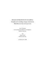
Figure 1.1 illustrates the use of module igrad1 for each north-south line of a topographic
map. We observe that the gradient gives an impression of illumination from a low sun angle.
To apply igrad1 along the 1-axis for each point on the 2-axis of a two-dimensional map, we
use the loop
1.1. FAMILIAR OPERATORS
7
Figure 1.1: Topography near Stanford (top) southward slope (bottom). ajt-stangrad90
[ER,M]