- Trang chủ >>
- Khoa Học Tự Nhiên >>
- Vật lý
Mathematical models in isotope hydrogeology iaea
Bạn đang xem bản rút gọn của tài liệu. Xem và tải ngay bản đầy đủ của tài liệu tại đây (15.1 MB, 207 trang )
IAEA-TECDOC-910
Manual
on
mathematical
models
in
isotope
hydrogeology
»
/-Snvb
»
INTERNATIONAL
ATOMIC
ENERGY
AGENCY
/A\
The
IAEA
does
not
normally maintain
stocks
of
reports
in
this
series.
However,
microfiche
copies
of
these
reports
can be
obtained
from
IN IS
Clearinghouse
International
Atomic
Energy
Agency
Wagramerstrasse
5
P.O.
Box 100
A-1400
Vienna,
Austria
Orders
should
be
accompanied
by
prepayment
of
Austrian
Schillings
100,-
in the
form
of a
cheque
or in the
form
of
IAEA
microfiche
service
coupons
which
may be
ordered
separately
from
the IN IS
Clearinghouse.
The
originating
Section
of
this
publication
in the
IAEA
was:
Isotope
Hydrology
Section
International
Atomic
Energy
Agency
Wagramerstrasse
5
P.O.
Box 100
A-1400
Vienna,
Austria
MANUAL
ON
MATHEMATICAL
MODELS
IN
ISOTOPE
HYDROGEOLOGY
IAEA,
VIENNA,
1996
IAEA-TECDOC-910
ISSN
1011-4289
©
IAEA,
1996
Printed
by the
IAEA
in
Austria
October
1996
FOREWORD
Methodologies
based
on the use of
naturally
occurring
isotopes
are,
at
present,
an
integral
part
of
studies
being
undertaken
for
water
resources
assessment
and
management.
Applications
of
isotope
methods
aim at
providing
an
improved
understanding
of the
overall
hydrological
system
as
well
as
estimating
physical
parameters
of the
system
related
to
flow
dynamics.
Quantitative
evaluations
based
on the
temporal
and/or
spatial
distribution
of
different
isotopic
species
in
hydrological
systems
require
conceptual
mathematical
formulations.
Different
types
of
model
can be
employed
depending
on the
nature
of the
hydrological
system
under
investigation,
the
amount
and
type
of
data
available,
and the
required
accuracy
of the
parameter
to be
estimated.
Water
resources
assessment
and
management requires
a
multidisciplinary
approach
involving
chemists,
physicists,
hydrologists
and
geologists.
Existing
modelling
procedures
for
quantitative
interpretation
of
isotope
data
are not
readily
available
to
practitioners
from
diverse
professional
backgrounds.
Recognizing
the
need
for
guidance
on the use of
different
modelling
procedures
relevant
to
specific
isotope
and/or
hydrological
systems,
the
IAEA
has
undertaken
the
preparation
of a
publication
for
this
purpose.
This
manual
provides
an
overview
of the
basic
concepts
of
existing
modelling
approaches,
procedures
for
their
application
to
different
hydrological
systems,
their
limitations
and
data
requirements.
Guidance
in
their
practical
applications,
illustrative
case
studies
and
information
on
existing
PC
software
are
also
included.
While
the
subject
matter
of
isotope
transport
modelling
and
improved
quantitative
evaluations
through
natural
isotopes
in
water
sciences
is
still
at the
development
stage,
this
manual
summarizes
the
methodologies
available
at
present,
to
assist
the
practitioner
hi the
proper
use
within
the
framework
of
ongoing
isotope
hydrological
field
studies.
In
view
of the
widespread
use of
isotope
methods
in
groundwater
hydrology,
the
methodologies covered
in the
manual
are
directed
towards
hydrogeological
applications,
although
most
of the
conceptual
formulations
presented
would
generally
be
valid.
Y.
Yurtsever,
Division
of
Physical
and
Chemical
Sciences,
was the
IAEA
technical
officer
responsible
for the
final
compilation
of
this
report.
It
is
expected
that
the
manual
will
be a
useful
guidance
to
scientists
and
practitioners
involved
in
isotope
hydrological applications,
particularly
in
quantitative
evaluation
of
isotope
data
in
groundwater
systems.
EDITORIAL
NOTE
In
preparing
this
publication
for
press,
staff
of the
IAEA
have
made
up the
pages
from
the
original
manuscripts
as
submitted
by the
authors.
The
views
expressed
do not
necessarily
reflect
those
of
the
governments
of the
nominating
Member
States
or
of
the
nominating
organizations.
Throughout
the
text
names
of
Member
States
are
retained
as
they
were
when
the
text
was
compiled.
The
use
of
particular
designations
of
countries
or
territories
does
not
imply
any
judgement
by
the
publisher,
the
IAEA,
as to the
legal
status
of
such
countries
or
territories,
of
their
authorities
and
institutions
or
of
the
delimitation
of
their
boundaries.
The
mention
of
names
of
specific
companies
or
products
(whether
or not
indicated
as
registered)
does
not
imply
any
intention
to
infringe
proprietary
rights,
nor
should
it be
construed
as an
endorsement
or
recommendation
on the
part
of
the
IAEA.
The
authors
are
responsible
for
having
obtained
the
necessary
permission
for the
IAEA
to
reproduce,
translate
or use
material
from
sources
already
protected
by
copyrights.
CONTENTS
SUMMARY
Lumped
parameter
models
for
interpretation
of
environmental
tracer
data
9
P.
Maloszewski,
A.
Zuber
Numerical
models
of
groundwater
flow
for
transport
59
L.F.
Konikow
Quantitative
evaluation
of
flow
systems,
groundwater
recharge
and
transmissivities
using
environmental
traces
.
113
EM.Adar
Basic
concepts
and
formulations
for
isotope
geochemical
modelling
of
groundwater
systems
155
R.M.
Kalin
List
of
related
IAEA
publications
207
SUMMARY
The
IAEA
has,
during
the
last
decade,
been
actively
involved
in
providing
support
to
development
and
field
verification
of the
various
modelling
approaches
in
order
to
improve
the
capabilities
of
modelling
for
reliable
quantitative
estimates
of
hydrological
parameters
related
to the
dynamics
of the
hydrological
system.
A
Co-ordinated
Research
Programme
(CRP)
on
Mathematical
Models
for
Quantitative
Evaluation
of
Isotope
Data
in
Hydrology
was
implemented
during
1990-1994.
The
results
of
this
CRP
were
published
as
IAEA-TECDOC-
777,
in
which
the
present
state-of-the-art
in
modelling
concepts
and
procedures
with
results
obtained
from
applied
field
research
are
summarized.
The
present
publication
is a
follow-up
to
the
earlier
work
and can be
considered
to be a
supplement
to
TECDOC-777.
Methodologies
based
on the use of
environmental
(naturally
occurring)
isotopes
are
being
routinely
employed
in the
field
of
water
resources
and
related
environmental
investigations.
Temporal
and/or
spatial
variations
of
commonly
used
natural
isotopes
(i.e.
stable
isotopes
of
hydrogen,
oxygen
and
carbon;
radioactive
isotopes
of
hydrogen
and
carbon)
in
hydrological
systems
are
often
employed
for two
main
purposes:
(i)
improved
understanding
of the
system
boundaries,
origin
(genesis)
of
water,
hydraulic
interconnections
between
different
sub-systems,
confirmation
(or
rejection)
of
boundary
conditions
postulated
as a
result
of
conventional
hydrological
investigations;
(ii)
quantitative
estimation
of
dynamic
parameters
related
to
water
movement
such
as
travel
time
of
water
and its
distribution
in the
hydrological
system,
mixing
ratios
of
waters
originating
from
different
sources
and
dispersion
characteristics
of
mass
transport
within
the
system.
Methodologies
of
isotope
data
evaluations
(as in i)
above)
are
essentially
based
on
statistical
analyses
of the
data
(either
in the
time
or the
space
domain)
which
would
contribute
to the
qualitative
understanding
of the
processes
involved
in the
occurrence
and
circulation
of
water,
while
the
quantitative
evaluations,
as in
(ii)
above,
would
require
proper
conceptual
mathematical
models
to be
used
for
establishing
the
link
between
the
isotopic
properties
with
those
of the
system
parameters.
The
general
modelling
approaches
developed
so far and
verified
through
field
applications
for
quantitative
interpretations
of
isotope
data
in
hydrology
cover
the
following
general
formulations:
Lumped
parameter
models,
that
are
based
on the
isotope
input-output
relationships
(transfer
function
models)
in the
tune
domain,
Distributed
parameter
numerical
flow
and
transport
models
for
natural
systems
with
complex
geometries
and
boundary
conditions,
Compartmental
models
(mixing
cell
models),
as
quasi-physical
flow
and
transport
of
isotopes
in
hydrological
systems,
Models
for
geochemical
speciation
of
water
and
transport
of
isotopes
with
coupled
geochemical
reactions.
While
the
modelling
approaches
cited
above
are
still
at a
stage
of
progressive
development
and
refinement,
the
IAEA
has
taken
the
initiative
for the
preparation
of
guidance
material
on the use of
existing
modelling
approaches
hi
isotope
hydrology.
The
need
for
such
a
manual
on the
basic
formulations
of
existing
modelling
approaches
and
their
practical
use
for
isotope
data
obtained
from
field
studies
was
recognized
during
the
deliberations
of the
earlier
CRP
mentioned
above.
Other
relevant
IAEA
publications
available
in
this
field
are
listed
at the end of
this
publication.
Use
of
specific
models
included
hi
each
of the
available
general
methodologies,
and
data
requirements
for
their
proper
use
will
be
dictated
by
many
factors,
mainly
related
to the
type
of
hydrological
system
under
consideration,
availability
of
basic
knowledge
and
scale
of
the
system.
Groundwater
systems
are
often
much
more
complex
in
this
regard,
and use of
isotopes
is
much
more
widespread
for a
large
spectrum
of
hydrological
problems
associated
with
proper
assessment
and
management
of
groundwater
resources.
Therefore,
this
manual,
providing
guidance
on the
modelling
approaches
for
isotope
data
evaluations,
is
limited
to
hydrogeological
applications.
Further
developments
required
in
this
field
include
the
following
specific
areas:
use of
isotopes
for
calibration
of
continuum
and
mixing-cell
models,
incorporation
of
geochemical
processes
during
isotope
transport,
particularly
for
kinetic
controlled
reactions,
improved
modelling
of
isotope
transport
in the
unsaturated
zone
and
models
coupling
unsaturated
and
saturated
flow,
stochastic
modelling
approaches
for
isotope
transport
and
their
field
verification
for
different
types
of
aquifers
(porous,
fractured).
The
IAEA
is
presently
implementing
a new CRP
entitled
"Use
of
Isotopes
for
Analyses
of
Flow
and
Transport
Dynamics
in
Groundwater
Systems",
which
addresses
some
of
the
above
required
developments
in
this
field.
Results
of
this
CRP
will
be
compiled
upon
its
completion
hi
1998.
While
the ami for the
preparation
of the
manual
was
mainly
to
provide
practical
guidance
on the
existing
modelling
applications
in
isotope
data
interpretations
for
water
resources
systems,
and
particularly
for
groundwater
systems,
the
methodologies
presented
will
also
be
relevant
to
environmental
studies
in
hydro-ecological
systems
dealing
with
pollutant
transport
and
assessment
of
waste
sites
(toxic
or
radioactive).
ii
mi
iBIII
inn mil
iiIII
Bill!
(0
XA9643080
LUMPED
PARAMETER
MODELS
FOR THE
INTERPRETATION
OF
ENVIRONMENTAL
TRACER
DATA
P.
MALOSZEWSKI
GSF-Institute
for
Hydrology
Oberschleissheim,
Germany
A
ZUBER
Institute
of
Nuclear
Physics,
Cracow,
Poland
Abstract
Principles
of the
lumped-parameter
approach
to the
interpretation
of
environmental
tracer
data
are
given.
The
following
models
are
considered:
the
piston
flow
model
(PFM),
exponential
flow
model
(EM),
linear
model
(LM),
combined
piston
flow
and
exponential
flow
model
(EPM),
combined
linear
flow
and
piston
flow
model
(LPM),
and
dispersion
model
(DM).
The
applicability
of
these
models
for the
interpretation
of
different
tracer
data
is
discussed
for a
steady
state
flow
approximation.
Case
studies
are
given
to
exemplify
the
applicability
of the
lumped-parameter
approach.
Description
of a
user-friendly
computer
program
is
given.
1.
Introduction
1.1.
Scope
and
history
of the
lamped-parameter
approach
This
manual
deals
with
the
lumped-parameter
approach
to the
interpreta-
tion
of
environmental
tracer
data
in
aquifers.
In a
lumped-parameter
model
or
a
black-box
model,
the
system
is
treated
as a
whole
and the
flow
pattern
is
assumed
to be
constant.
Lumped-parameter
models
are the
simplest
and
best
applicable
to
systems
containing
young
water
with
modern
tracers
of
variable
input
concentrations,
e.g.,
tritium,
Kr-85
and
freons,
or
seasonably
varia-
ble
0 and
2
H. The
concentration
records
at the
recharge
area
must
be
known
or
estimated,
and for
measured
concentrations
at
outflows
(e.g.
springs
and
abstraction
wells),
the
global
parameters
of the
investigated
system
are
found
by a
trial-and-error
procedure.
Several
simple
models
commonly
applied
to
large
systems
with
a
constant
tracer
input
(e.g.
the
piston
flow
model
usually
applied
to the
interpretation
of
radiocarbon
data)
also
belong
to
the
category
of the
lumped-parameter
approach
and are
derivable
from
the
general
formula.
The
manual
contains
basic
definitions
related
to the
tracer
method,
outline
of the
lumped-parameter
approach,
discussion
of
different
types
of
flow
models
represented
by
system
response
functions,
definitions
and
dis-
cussion
of the
parameters
of the
response
functions,
and
selected
case
studies.
The
case
studies
are
given
to
demonstrate
the
following
problems:
difficulties
in
obtaining
a
unique
calibration,
relation
of
tracer
ages
to
flow
and
rock
parameters
in
granular
and
fissured
systems,
application
of
different
tracers
to
some
complex
systems.
Appendix
A
contains
examples
of
response
functions
for
different
injection-detection
modes.
Appendix
B
contains
an
example
of
differences
between
the
water
age,
the
conservative
tracer
age,
and the
radioisotope
age
"for
a
fissured
aquifer.
Appendix
C
contains
user's
guide
to the
FLOW
- a
computer
program
for the
interpreta-
tion
of
environmental
tracer
data
in
aquifers
by the
lumped-parameter
ap-
proach,
which
is
supplied
on a
diskette.
[*]
The
interpretation
of
tracer
data
by the
lumped-parameter
approach
is
particularly
well
developed
in
chemical
engineering.
The
earliest
quantita-
tive
interpretations
of
environmental
tracer
data
for
groundwater
systems
were
based
on the
simplest
models,
i.e.,
either
the
piston
flow
model
or the
exponential
model
(mathematically
equivalent
to the
well-mixed
cell
model),
which
are
characterized
by a
single
parameter
[1].
A
little
more
sophisti-
cated
two-parameter
model,
represented
by
binomial
distribution
was
intro-
duced
in
late
1960s
[2].
Other
two-parameter
models,
i.e,
the
dispersion
model
characterized
by a
uni-dimensional
solution
to the
dispersion
equa-
tion,
and the
piston
flow
model
combined
with
the
exponential
model,
were
shown
to
yield
better
fits
to the
experimental
results
[3].
All
these
models
have
appeared
to be
useful
for
solving
a
number
of
practical
problems,
as it
will
be
discussed
in
sections
devoted
to
case
studies.
Recent
progress
in
numerical
methods
and
multi-level
samplers
focused
the
attention
of
model-
lers
on
two-
and
three-dimensional
solutions
to the
dispersion
equation.
However,
the
lumped-parameter
approach
still
remains
to be a
useful
tool
for
solving
a
number
of
practical
problems.
Unfortunately,
this
approach
is
often
ignored
by
some
investigators.
For
instance,
in a
recent
review
[4] a
general
description
of the
lumped-parameter
approach
was
completely
omitted,
though
the
piston
flow
and
well-mixed
cell
models
were
given.
The
knowledge
of
the
lumped-parameter
approach
and the
transport
of
tracer
in the
simplest
flow
system
is
essential
for a
proper
understanding
of the
tracer
method
and
possible
differences
between
flow
and
tracer
ages.
Therefore,
even
those
who
are not
interested
in the
lumped-parameter
approach
are
advised
to get ac-
quainted
with
the
following
text
and
particularly
with
the
definitions
given
below,
especially
as
some
of
these
definitions
are
also
directly
or
indi-
rectly
applicable
to
other
approaches.
1.2.
Useful
definitions
In
this
manual
we
shall
follow
definitions
taken
from
several
recent
publications
[5, 6, 7, 8, 9]
with
slight
modifications.
However,
it
must
be
remembered
that
these
definitions
are not
generally
accepted
and a
number
of
authors
apply
different
definitions,
particularly
in
respect
to
such
terms
as
model
verification
and
model
validation.
Therefore,
caution
is
needed,
and,
in the
case
of
possible
misunderstandings,
the
definitions
applied
should
be
either
given
or
referred
to an
easily
available
paper.
As far as
verification
and
validation
are
concerned
the
reader
is
also
referred
to
authors
who are
very
critical
about
these
terms
used
in
their
common
meaning
and
who are of a
opinion
that
they
should
be
rejected
as
being
highly
mis-
leading
[10, 11].
The
tracer
method
is a
technique
for
obtaining
information
about
a
sys-
tem
or
some
part
of a
system
by
observing
the
behaviour
of a
specified
sub-
stance,
the
tracer,
that
has
been
added
to the
system.
Environmental
tracers
are
added
(injected)
to the
system
by
natural
processes,
whereas
their
pro-
duction
is
either
natural
or
results
from
the
global
activity
of
man.
[*]
User
Guide
and
diskette
are
available
free
of
charge
from
Isotope
Hydrology
Section,
IAEA,
Vienna,
upon
request.
10
An
ideal
tracer
is a
substance
that
behaves
in the
system
exactly
as
the
traced
material
as far as the
sought
parameters
are
concerned,
and
which
has one
property
that
distinguishes
it
from
the
traced
material.
This
defi-
nition
means
that
for an
ideal
tracer
there
should
be
neither
sources
nor
sinks
in the
system
other
than
those
adherent
to the
sought
parameters.
In
practice
we
shall
treat
as a
good
tracer
even
a
substance
which
has
other
sources
or
sinks
if
they
can be
properly
accounted
for,
or if
their
influ-
ence
is
negligible within
the
required
accuracy.
A
conceptual
model
is a
qualitative
description
of a
system
and its
representation
(e.g.
geometry,
parameters,
initial
and
boundary
conditions)
relevant
to the
intended
use of the
model.
A
mathematical
model
is a
mathematical
representation
of a
conceptual
model
for a
physical,
chemical,
and/or
biological
system
by
expressions
de-
signed
to aid in
understanding
and/or
predicting
the
behaviour
of the
system
under
specified
conditions.
Verification
of a
mathematical
model,
or its
computer
code,
is
obtained
when
it is
shown
that
the
model
behaves
as
intended,
i.e.
that
it is a
prop-
er
mathematical
representation
of the
conceptual
model
and
that
the
equa-
tions
are
correctly
encoded
and
solved.
A
model
should
be
verified
prior
to
calibration.
Model
calibration
is a
process
in
which
the
mathematical
model
assump-
tions
and
parameters
are
varied
to fit the
model
to
observations.
Usually,
calibration
is
carried
out by a
trial-and-error
procedure.
The
calibration
process
can be
quantitatively
described
by the
goodness
of
fit.
Model
calibration
is a
process
in
which
the
inverse
problem
is
solved,
i.e.
from
known
input-output
relations
the
values
of
parameters
are
deter-
mined
by
fitting
the
model
results
to
experimental
data.
The
direct
problem
is
solved
if for
known
or
assumed
parameters
the
output
results
are
calcu-
lated
(model
prediction).
Testing
of
hypotheses
is
performed
by
comparison
of
model
predictions
with
experimental
data.
Validation
is a
process
of
obtaining
assurance
that
a
model
is a
correct
representation
of the
process
or
system
for
which
it is
intended.
Ideally,
validation
is
obtained
if the
predictions
derived
from
a
calibrated
model
agree
with
new
observations,
preferably
for
other
conditions
than
those
used
for
calibration.
Contrary
to
calibration,
the
validation
process
is
a
qualitative
one
based
on the
modeller's
judgment.
The
term
"a
correct
representation"
may
perhaps
be
misleading
and too
much
promising.
Therefore,
a
somewhat
changed
definition
can be
proposed:
Validation
is a
process
of
obtaining
assurance
that
a
model
satisfies
the
modeller's
needs
for the
process
or
system
for
which
it is
intended,
within
an
assumed
or
requested
accuracy
[9].
A
model
which
was
validated
for
some
purposes
and at a
given
stage
of
investigations,
may
appear
invalidated
by
new
data
and
further
studies.
However,
this
neither
means
that
the
valida-
tion
process
should
not be
attempted,
nor
that
the
model
was
useless.
Partial
validation
can be
defined
as
validation
performed
with
respect
to
some
properties
of a
model
[7, 8]. For
instance,
models
represented
by
solutions
to the
transport
equation
yield
proper
solute
velocities
(i.e.
can
be
validated
in
that
respect
- a
partial
validation),
but
usually
do not
yield
proper
dispersivities
for
predictions
at
larger
scales.
In
the
case
of the
tracer
method
the
validation
is
often
performed
by
comparison
of the
values
of
parameters
obtained
from
the
models
with
those
obtainable
independently
(e.g.
flow
velocity
obtained
from
a
model
fitted
to
tracer
data
is
shown
to
agree
with
that
calculated
from
the
hydraulic
gra-
dient
and
conductivity
known
from
conventional
observations
[7, 8, 12,
13].
When
results
yielded
by a
model
agree
with
results
obtained
independently,
a
number
of
authors
state
that
the
model
is
confirmed,
e.g. [11],
which
is
equivalent
to the
definition
of
validation
applied
within
this
manual.
The
direct
problem
consists
in
finding
the
output
concentration
curve(s)
for
known
or
assumed
input
concentration,
and for
known
or
assumed
11
model
type
and its
parameter(s).
Solutions
to the
direct
problem
are
useful
.for
estimating
the
potential
abilities
of the
method,
for
planning
the
fre-
quency
of
sampling,
and
sometimes
for
preliminary
interpretation
of
data,
as
explained
below.
The
inverse problem
consists
in
searching
for the
model
of a
given
sys-
tem
for
which
the
input
and
output
concentrations
are
known.
Of
course,
for
this
purpose
the
graphs
representing
the
solutions
to the
direct
problem
can
be
very
helpful.
In
such
a
case
the
graph
which
can be
identified with
the
experimental
data
will
represent
the
solution
to the
inverse
problem.
A
more
proper
way is
realized
by
searching
for the
best
fit
model
(calibration).
Of
course,
a
good
fit is a
necessary
condition
but not a
sufficient
one to
con-
sider
the
model
to be
validated
(confirmed).
The
fitting
procedure
has to be
used
together
with
the
geological
knowledge,
logic
and
intuition
of the
mod-
eller
[14].
This
means
that
all the
available
information
should
be
used
in
selecting
a
proper
type
of the
model
prior
to the
fitting.
If the
selection
is
not
possible
prior
to the
fitting,
and if
more
than
one
model
give
equal-
ly
good
fit but
with
different
values
of
parameters,
the
selection
has to be
performed
after
the
fitting,
as a
part
of the
validation
process.
It is a
common
sin of
modellers
to be
satisfied
with
the fit
obtained
without
check-
ing
if
other
equally
good
fits
are not
available.
In
dispersive
dynamic
systems,
as
aquifers,
it is
necessary
to
distin-
guish
between
different
ways
in
which
solute
(tracer)
concentration
can be
measured.
The
resident
concentration
(C )
expresses
the
mass
of
solute
(Am)
R
per
unit
volume
of
fluid
(AV)
contained
in a
given
element
of the
system
at
a
given
instant,
t:
C (t) =
Am(t)/AV
(1)
R
The
flux
concentration
(C )
expresses
the
ratio
of the
solute
flux
(Am/At)
to the
volumetric fluid
flow
(Q =
AV/At)
passing
through
a
given
cross-section:
Am(t)/At
Am(t)
F
AV/At
QAU)
l J
The
resident
concentration
can be
regarded
as the
mean
concentration
obtained
by
weighting over
a
given
cross-section
of the
system,
whereas
the
flux
concentration
is the
mean
concentration
obtained
by
weighting
by the
volumetric
flow
rates
of
flow
lines
through
a
given
cross-section
of the
system.
The
differences
between
two
types
of
concentration
were
shown
either
theoretically
or
experimentally
by a
number
of
authors
[15,
16, 17,
18].
However,
numerical
differences
between
both
types
of
concentration
are of
importance
only
for
laminar
flow
in
capillaries
and for
highly
dispersive
systems
[18,
19]
(see
Appendix
A).
The
turnover
time
or age of
water
leaving
the
system
(t ) is
defined
w
as:
t
= V /Q
(3a)
w
m
where
V is the
volume
of
mobile
water
in the
system.
For
systems
which
can
be
approximated
by
unidimensional
flow,
Eq. 3
reads:
Sn
x
t
= v /Q =
F
-^—
= —
(3b)
w
m Sn v v
12
where
x is the
length
of the
system
measured
along
the
streamlines,
v is
the
mean
velocity
of
water,
n is the
space
fraction
occupied
by the
mobile
water
(effective
porosity),
and S is the
cross-section
area
normal
to
flow.
According
to Eq. 3b, the
mean
water
velocity
is
defined
as:
v
=
Q/(n
S) = v /n (4)
w
e f e
where
v is
Darcy's
velocity
defined
as
Q/S.
2.
Immobile
systems
Discussion
of
immobile
systems
is
beyond
the
scope
of
this
manual,
but
for
the
consistency
of the age
definitions
they
are
briefly
discussed
below.
For
old
groundwaters,
a
distinction
should
be
made
between
mobile
and
immo-
bile
systems,
especially
in
respect
to the
definition
of
age.
A
radioisotope
tracer,
which
has no
other
source
and
sink
than
the
radioactive
decay,
rep-
resents
the age of
water
in an
immobile
system,
if the
system
is
separated
from
recharge
and the
mass
transfer
with
adjacent
systems
by
molecular
diffusion
is
negligible.
Then
the
radioisotope
age (t ),
understood
as the
fl
time
span
since
the
separation
event,
is
defined
by the
well
known
formula
of
the
radioactive
decay,
and it
should
be the
same
in the
whole
system:
C/C(0)
=
exp(-At
) (5)
A
where
C and
C(0)
are the
actual
and
initial
radioisotope
concentrations,
and
A
is the
radioactive
decay
constant.
Unfortunately,
ideal
radioisotope
tracers
are not
available
for
dating
of
old
immobile
water
systems.
Therefore,
we
shall
mention
that
the
accumu-
lation
of
some
tracers
is a
more
convenient
tool,
if the
accumulation
rate
can be
estimated
from
the in
situ
production
and the
crust
or
mantle
flux
as
4 40
it
is in the
case
of He and AT
dating
for
both
mobile
and
immobile
sys-
tems.
Similarly,
the
dependence
of H and 0
contents
in
water
molecules
on
the
climatic
conditions
of
recharge
during
different
geological
periods
as
well
as
noble
gas
concentrations
expressed
in
terms
of the
temperature
at
the
recharge
area
(noble
gas
temperatures)
may
also
serve
for
reliable
trac-
ing
of
immobile
groundwater
systems
in
terms
of
ages.
3.
Basic
principles
for
constant
flow
systems
The
exit
age-distribution
function,
or the
transit
time
distribution,
E(t), describes
the
exit
time
distribution
of
incompressible
fluid
elements
of the
system
(water)
which
entered
the
system
at a
given
t = 0.
This
func-
tion
is
normalized
in
such
a way
that:
00
E(t)
dt = 1 (6)
0
I
According
to the
definition
of the
E(t)
function,
the
mean
age of
water
leaving
the
system
is:
00
t
= f
tE(t)
dt (7)
w J
13
The
mean
transit
time
of a
tracer
(t ) or the
mean
age of
tracer
is
defined
as:
00 00
t
= f 1C (t) dt / f C (t) dt
(8~.
t J I J 1
where
C (t) is the
tracer
concentration
observed
at the
measuring
point
as
the
result
of an
instantaneous
injection
at the
injection
point
at t = 0.
Equation
8
defines
the age of any
tracer
injected
and
measured
in any
mode.
In
order
to
avoid
possible
misunderstandings,
in all
further
considerations,
t
denotes
the
mean
age of a
conservative
tracer.
Unfortunately,
it is a
common
mistake
to
identify
Eq. 7
with
Eq. 8 for
conservative
tracers
(or for
radioisotope
tracers
corrected
for the
decay)
whereas
the
mean
age of a
con-
servative
tracer
leaving
the
system
is
equal
to the
mean
age of
water
only
if
the
tracer
is
injected
and
measured
in the
flux
mode
and if no
stagnant
water
zones
exist
in the
system.
Consequently,
because
the
tracer
age may
differ
from
the
water
age,
it is
convenient
to
define
a
function
describing
the
distribution
of a
conservative
tracer.
This
function,
called
the
weight-
ing
function,
or the
system
response
function,
g(t),
describes
the
exit
age-
distribution
of
tracer
particles
which
entered
the
system
of a
constant
flow
rate
at a
given
t = 0:
g(t)
=
C^tJ/
C
:
(t)
dt =
cyUQ/M
(9)
0
because
the
whole
injected
mass
or
activity
(M) of the
tracer
has to
appear
at
the
outlet,
i.e.:
CO
M
= Q J
C^t)
dt
(10)
0
As
mentioned,
the
g(t)
function
is
equal
to the
E(t)
function,
and,
consequently,
the
mean
age of
tracer
is
equal
to the
turnover
time
of
water,
if
a
conservative
tracer
(or a
decaying
tracer
corrected
for the
decay)
is
injected
and
measured
in the
flux
mode,
and if
there
are no
stagnant
zones
in
the
system.
Systems
with
stagnant
zones
are
discussed
in
Sect.
9. In the
lumped-parameter
approach
it is
usually
assumed
that
the
concentrations
are
observed
in
water
entering
and
leaving
the
system,
which
means
that
flux
concentrations
are
applicable.
Therefore,
in all
further
considerations
the
C
symbol
stays
for
flux
concentrations,
and the
mean
transit
time
of
tracer
is
equal
to the
mean
transit
time
of
water
unless
stated
otherwise.
Equation
8 is of
importance
in
artificial
tracing,
and,
together
with
Eq.
9,
serves
for
theoretical
findings
of the
response
functions
in
environ-
mental
tracing.
For a
steady
flow
through
a
groundwater
system,
the
output
concentration,
C(t),
can be
related
to the
input
concentration
(C ) of any
in
tracer
by the
well
known
convolution
integral:
C(t)
=
("c
(t-f)
g(t')
exp(-At')
dt'
(lla)
J
in
14
where
t' is the
transit
time,
or
0
C(t)
= \ C
it')
g(t-t')
expt-A(t-t')
df
(lib)
J
in
-co
where
t' is
time
of
entry,
and
t-t'
is the
transit
time.
The
type
of the
model
(e.g.
the
piston
flow
model,
or
dispersion
model)
is
defined
by the
g(t')
function
chosen
by the
modeller
whereas
the
model
parameters
are to be
found
by
calibration
(fitting
of
concentrations
calculated
from
Eq. 11 to
experimental
data,
for
known
or
estimated
input
concentrat
ion
records).
4.
Models
and
their
parameters
4.1.
General
The
lumped-parameter
approach
is
usually
limited
to
one-
or
two-param-
eter
models.
However,
the
type
of the
model
and its
parameters
define
the
exit-age
distribution
function
(the
weighting
function)
which
gives
the
spectrum
of the
transit
times.
Therefore,
if the
modeller
gives
just
the
type
of the
model
and the
mean
age,
the
user
of the
data
can be
highly mis-
led.
Consider
for
instance
an
exponential
model
and the
mean
age of 50
years.
The
user
who has no
good
understanding
of the
models
may
start
to
look
for a
relatively
distant
recharge
area,
and may
think
that
there
is no
danger
of a
fast
contamination.
However,
the
exponential
model
(see
Sects
4.3 and
9.1)
means
that
the
flow
lines with extremely
short
(theoretically
equal
to
zero)
transit
times
exist.
Therefore,
the
best
practice
is to re-
port
both
the
parameters
obtained
and the
weighting
function
calculated
for
these
parameters. Another
possible
misunderstanding
is
also
related
to the
mean
age.
For
instance,
the
lack
of
tritium
means
that
no
water
recharged
in
the
hydrogen-bomb
era is
present
(i.e.,
after
1952).
However,
for
highly
dispersive
systems
(e.g.
those
described
by the
exponential
model
or the
dispersive
model
with
a
large
value
of the
dispersion
parameter),
the
pres-
ence
of
tritium
does
not
mean
that
an age of 100
years,
or
more,
is not
possible.
Sometimes
either
it is
necessary
to
assume
the
presence
of two
water
components
(e.g.,
in
river
bank
filtration
studies),
or it is
impossible
to
obtain
a
good
fit
(calibration)
without
such
an
assumption.
The
additional
parameter
is
denoted
as
ft,
and
defined
as the
fraction
of
total
water
flow
with
a
constant
tracer
concentration,
C
0
.
p
4.2.
Piston
Flow
Model
(PFM)
In
the
piston
flow
model
(PFM) approximation
it is
assumed
that
there
are no
flow
lines
with
different
transit
times,
and the
hydrodynamic
disper-
sion
as
well
as
molecular
diffusion
of the
tracer
are
negligible.
Thus
the
tracer
moves
from
the
recharge
area
as if it
were
in a
parcel.
The
weighting
function
is
given
by the
Dirac
delta
function
[g(f
) =
6(t'-t
)],
which
inserted
into
Eq. 9
gives:
C(t)
= C
(t-t
)
exp(-Xt
)
(12)
in
t t
Equation
12
means
that
the
tracer
which
entered
at a
given
time
t-t
leaves
the
system
at the
moment
t
with
concentration
decreased
by the
radio-
15
active
decay
during
the
time
span
t . The
mean
transit
time
of
tracer
(t )
equal
to the
mean
transit
time
of
water
(t ) is the
only
parameter
of
PFM.
w
Cases
in
which
t may
differ
from
t are
discussed
in
Sect.
9.
t
w
4.3.
Exponential
Model
(EH)
In
the
exponential
model
(EM)
approximation
it is
assumed
that
the
exponential
distribution
of
transit
times
exists,
i.e.,
the
shortest
line
has the
transit
time
of
zero
and the
longest
line
has the
transit
time
of
infinity.
Tracer
concentration
for an
instantaneous
injection
is: C (t) =
C (0)
exp(-t/t
).
This
equation
inserted
into
Eq. 9, and
normalized
in
such
a way
that
the
initial
concentration
is as if the
injected
mass
(M) was
diluted
in the
volume
of the
system
(V ),
gives:
m
g(t')
= t'
1
exp(-f/t
t
)
(13)
The
mean
transit
time
of
tracer
(t ) is the
only
parameter
of EM. The
exponential
model
is
mathematically
equivalent
to the
well
known
model
of
good
mixing
which
is
applicable
to
some
lakes
and
industrial
vessels.
A lot
of
misunderstandings
result
from
that
property.
Some
investigators
reject
the
exponential
model
because
there
is no
possibility
of
good
mixing
in
aquifers
whereas
others
claim
that
the
applicability
of the
model
indicates
conditions
for a
good
mixing
in the
aquifer.
Both
approaches
are
wrong
because
the
model
is
based
on an
assumption
that
no
exchange
(mixing)
of
tracer
takes
place
between
the
flow
lines
[1, 6, 8]. The
mixing
takes
place
only
at the
sampling
site
(spring,
river
or
abstraction
well).
That
problem
will
be
discussed
further.
A
normalized
weighting
function
for EM is
given
in
Fig.
1.
Note that
the
normalization
allows
to
represent
an
infinite
number
of
cases
by a
sin-
gle
curve.
In
order
to
obtain
the
weighting
function
in
real
time
it is
nec-
essary
to
assume
a
chosen
value
of t and
recalculate
the
curve
from
Fig.
1.
The
mean
transit
time
of
tracer
(t )
equal
to the
mean
transit
time
of
water
(t ) is the
only
parameter
of EM.
Cases
in
which
t may
differ
from
t
w t w
are
discussed
in
Sect.
9.
4.4.
Linear
Model
(LM)
In
the
linear
model
(LM)
approximation
it is
assumed
that
the
distribu-
tion
of
transit
times
is
constant,
i.e.,
all the
flow
lines
have
the
same
velocity
but
linearly
increasing
flow
time.
Similarly
to EM,
there
is no
mixing
between
the
flow
lines.
The
mixed
sample
is
taken
in a
spring,
river,
or
abstraction
well
[1, 3, 6]. The
weighting
function
is:
g(t)
=
l/(2t
) for t' == 2t
(14)
= 0 for t' 2: 2t
The
mean
transit
time
of
tracer
(t ) is the
only
parameter
of LM. A
normalized
weighting
function
is
given
in
Fig.
2. In
order
to
obtain
the
weighting
function
in
real
time
it is
necessary
to
assume
a
chosen
value
of
t
and
recalculate
the
curve
from
Fig.
2.
16
The
mean
transit
time
of
tracer
(t )
equal
to the
mean
transit
time
of
water
(t ) is the
only
parameter
of LM.
Cases
in
which
t may
differ
from
t
w t w
are
discussed
in
Sect.
9.
4.5.
Combined
Exponential-Piston
Flow
Model
(EPM)
In
general
it is
unrealistic
to
expect
that single-parameter
models
can
adequately describe
real
systems,
and,
therefore,
a
little
more
realistic
two-parameter
models
have
also
been
introduced.
In the
exponential-piston
model
it is
assumed
that
the
aquifer
consists
of two
parts
in
line,
one
with
the
exponential
distribution
of
transit
times,
and
another
with
the
distri-
bution
approximated
by the
piston
flow.
The
weighting
function
of
this
model
is
[3, 6]:
g(t')
=
(Vt
fc
)
exp(-7)t'/t
t
+
=
0
- 1)
for t' 2: t (1 -
15)
1
for t' < t (1 - if)
where
T) is the
ratio
of the
total
volume
to the
volume
with
the
exponential
distribution
of
transit
times,
i.e.,
T) = 1
means
the
exponential
flow
model
(EM).
The
model
has two
fitting
(sought)
parameters,
t and T). The
weighting
function
does
not
depend
on the
order
in
which
EM and PFM are
combined.
An
example
of a
normalized
weighting
function
obtained
for 7) = 1.5 is
given
in
Fig.
1.
However, experience
shows
that
EPM
works
well
for T)
values
slightly
larger
than
1,
e.i.,
for a
dominating
exponential flow pattern
corrected
for
the
presence
of a
small
piston
flow
reservoir.
In
other
cases,
DM is
more
adequate.
In
order
to
obtain
the
weighting function
for a
given
value
of T> and a
chosen
t
value
in
real
time
it is
necessary
to
recalculate
the
curve
from
Fig.
1.
Cases
in
which
t may
differ
from
t are
discussed
in
Sect.
9.
1
2
NORMALIZED
TIME
,
t'/t,
Fig.
I. The
g(t')
function
of EM, and the
g(t')
function
of EPM in the
case
of T) = 1.5 [3, 6].
17
4.6.
Combined
Linear-Piston
Flow
Model
(LPM)
The
combination
of LM
with
PFM
gives
similarly
to EPM the
linear-piston
model
(LPM).
Similarly
to EPM the
weighting
function
has two
parameters
and
does
not
depend
on the
order
in
which
the
models
are
combined.
The
weighting
function
is [3, 6]:
g(t')
=
=
0
t
- t /I) £ t'
for
for
other
t'
+
t
t
/T)
(16)
where
T> is the
ratio
of the
total
volume
to the
volume
in
which
linear
flow
model
applies,
i.e.,
TJ = 1.0
means
the
linear
flow
model
(LM).
An
example
of
the
weighting
function
is
given
in
Fig.
2.
Weighting
functions
in
real
time
are
obtainable
in the
same
way as
described
above
for
other
models.
Cases
in
which
t
differs
from
t
t
are
discussed
in
Sect.
9.
4.7.
Dispersion
Model
(DM)
In the
dispersion
model
(DM)
the
uni-dimensional
solution
to the
dis-
persion
equation
for a
semi-infinite
medium
and
flux
injection-detection
mode,
developed
in
[20]
and
fully
explained
in
[18],
is
usually
put
into
Eq.
9
to'obtain
the
weighting
function,
though
sometimes
other
approximations
are
also
applied.
That
weighting
function
reads
[3, 6]:
g(t')
=
(4ITt'
3
/Pet
t
r
1/2
exp[-(l
-
(17)
where
Pe is the
so-called
Peclet
number.
The
reciprocal
of Pe is
equal
to
the
dispersion
parameter,
Pe
-1
= D/vx,
where
D is the
dispersion
coefficient.
In
the
lumped
parameter
approach
the
dispersion
parameter
is
treated
as a
single
parameter.
The
meaning
of
that
parameter
is
discussed
in
Sect.
9.1.
1.O
-OS
o>
i
T r
i
i i i n r
LPM for
tx=1.5
LM
i/r
' I
,
\l .
0 t 2
NORMALIZED
TIME
,
f/t,
Fig.
2. The
g(t')
function
of LM, and the
g(t')
function
of LPM in the
case
of T) = 1.5 [3, 61.
18
5.0
0.2
0.6 . 0.8 1.0 1.2
NORMALIZED
TRANSIT
TIME
t'/t,
1.6
1.8
Fig.
3.
Examples
of the
g(t')
functions
for DM in
flux
mode
[3, 6]. The
g(t')
function
of EM is
shown
for
comparison.
Examples
of
normalized
weighting
functions
for DM in the
flux
mode
are
shown
in
Fig.
3.
Weighting
functions
in
real
time
are
obtainable
in the
same
way as
described
above
for
other
models.
Cases
in
which
t
differs
from
t
t
w
are
discussed
in
Sect.
9.
The
dispersion
model
can
also
be
applied
for the
detection
performed
in
the
resident
concentration
mode
(see
Eq. 1).
Then
the
weighting
function
reads
[3, 6]:
— 1 /^?
—
g(t')
=
{(TTt'/Pet
)
exp[-(l
-
t'/t
) t
Pe/f
] -
W W W
—
1 /^
(Pe/2)
exp(Pe)
erfc[(l
+
t'/t
)(4t'/Pet
)
]>/t
w w »
(18)
where
erfc(z)
= 1 -
erf(z),
erf(z)
being
the
tabulated
error
function.
In
the
case
of Eq. 18 the
mean
transit
time
of
tracer
always
differs
from
the
mean
transit
time
of
tracer
and in
ideal
cases
is
given
by: t = (1 +
Pe )t ,
which
shows
that
even
if
there
are no
stagnant
zones
in the
system
19
the
mean
transit
time
of a
conservative
tracer
may
differ
from
the
mean
transit
time
of
water.
Cases
of
stagnant
water
zones
are
discussed
in
Sects
9.2 and
9.3.
A
misunderstanding
is
possible
as a
result
of
different
applications
of
the
dispersion
equation
and its
solutions.
For
instance,
in the
pollutant
movement
studies
the
dispersion
equation
usually
serves
as a
distributed
parameter
model,
especially
when
numerical
solutions
are
used.
Then,
the
dispersion
coefficient
(or the
dispersivity,
D/v,
or
dispersion
parameter,
Pe ,
depending
on the way in
which
the
solutions
are
presented)
represents
the
dispersive
properties
of the
rock.
If the
dispersion
model
is
used
in
the
lumped
parameter
approach
for the
interpretation
of
environmental
data
in
aquifers,
the
dispersion
parameter
is an
apparent
quantity
which
mainly
depends
on the
distribution
of
flow
transit
times,
and is
practically
order
of
magnitudes
larger
than
the
dispersion
parameter
resulting
from
the
hydro-
dynamic
dispersion,
as
explained
in
Sect.
9.1.
However,
in the
studies
of
vertical
movement
through
the
unsaturated
zone,
or in
some
cases
of
river
bank
infiltration,
the
dispersion
parameter
can be
related
the
hydrodynamic
dispersion.
5.
Cases
of
constant
tracer
input
For
radioisotope
tracers,
the
cases
of a
constant
input
can be
solved
analytically.
They
are
applicable
mainly
to C and
tritium
prior
to
atmos-
pheric
fusion-bomb
tests
in the
early
1950s.
The
following
solutions
are
obtainable
from
Eq. 9 [1, 3, 6]:
C
= C
exp(-A/t
) for PFM
(19)
0 a
C
= C /(I + A/t ) for EM
(20)
O
a
C = C [1 -
exp(-2At
)]/(2At
) for LM
(21)
0 a a
—1
1 /^
C = C
exp{(Pe/2)x[l
- (1 + 4At Pe ) ]} for DM
(22)
0 a
where
C is a
constant
concentration
measured
in
water
entering
the
system
and t is
replaced
by t
(radioisotope
age)
to the
reasons
discussed
in
W A
detail
in
Sect.
9.
Here,
we
shall
remind
only
that
for
nonsorbable
tracers
and
systems
without
stagnant
zones
t = t .
Unfortunately,
it is a
common
W
3
mistake
to
identify
the
radiocarbon
age
obtained
from
Eq. 19
with
the
water
age
without
any
information
if PFM is
applicable
and if the
radiocarbon
is
not
delayed
by
interaction
between
dissolved
and
solid
carbonates.
Relative
concentration
(C/C
)
given
as
functions
of
normalized
time
(At
) are
given
in
Fig.
4
(for
tritium
I/A =
17.9
a, and for
radiocarbon
I/A
A
=
8,300
a).
From
Eqs 19 to 22 and
Fig.
4,
several
conclusions
can
immediate-
ly
be
drawn.
First,
for a
sample
taken
from
a
well,
it is in
principle
not
possible
to
distinguish
if the
system
is
mobile
or
immobile
(however,
if a
short-lived
radioisotope
is
present,
it
would
be
unreasonable
to
assume
that
the
system
can be
separated
from
the
recharge).
Second,
the
applicability
of
the
piston
flow
model
(PFM)
is
justified
for a
constant
tracer
input
to
sys-
tems
with
the
values
of the
dispersion
parameter,
say,
not
larger
than
about
0.05.
Third,
from
the
measured
C/C
ratio
it is not
possible
to
obtain
the
radioisotope
age
without
the
knowledge
on the
model
of
flow
pattern
even
if
a
single-parameter
model
is
assumed.
Fourth,
for
ages
below,
say,
0.5(1/A),
20
c
0
Z
o
z
UJ
o
o
UJ
UJ
a;
QOOS
0.05
-
0.01
-
0.2
0.5
1.0 5 10
RELATIVE
TURNOVER
TIME,Xt,
100
Fig.
4.
Relative
concentration
versus
relative
radioisotope
age (At ), in
the
case
of a
constant
input
of a
radioactive
tracer
[3, 6]. EM -
exponen-
tial
model,
LM -
linear
model,
PFM -
piston
flow
model,
Pe~ -
dispersion
parameter
for the
dispersion
model
in the
flux
mode.
the
flow
pattern
(type
of
model)
has low
influence
on the age
obtained.
Fifth,
for
two-parameter
models
it is
impossible
to
obtain
the age
value
(it
is
like
solving
a
single
equation
with
two
unknowns).
When
no
information
is
available
on the
flow
pattern,
the
ages
obtained
from
PFM and EM can
serve
as
brackets
for
real
values,
though
in
some
ex-
treme
cases
DM can
yield
higher
ages
(see
Fig.
4).
Radioisotopes
with
a
constant
input
are
applicable
as
tracers
for the
age
determination
due to the
existence
of a
sink
(radioactive
decay),
which
is
adherent
to the
sought
parameter
(see
the
definition
of an
ideal
tracer
in
Sect.
1.2).
Other
substances
cannot
serve
as
tracers
for
this
purpose
though
they
come
under
earlier
definitions
of an
ideal
tracer.
However,
those
other
substances
(e.g.,
Cl~)
may
serve
as
good
tracers
for
other
pur-
poses,
e.g.,
for
determining
the
mixing
ratio
of
different
waters.
Note
that
for a
constant
tracer
input,
a
single
determination
serves
for the
calculation
of
age.
Therefore,
no
calibration
can be
performed.
The
only
way to
validate,
or
confirm,
a
model
is to
compare
its
results
with
other
independent
data,
if
available.
21
6.
Cases
of
variable
tracer
input
6.1.
Tritium
method
Seasonal
variations
of the
tritium
concentration
in
precipitation
cause
serious
difficulties
in
calculating
the
input
function,
C
(t).
The
best
in
method would
be to
estimate
for
each
year
the
mean
concentration
weighted
by
the
infiltration
rates:
12 12
C.
= y
C.cc.P./
y a P
(23)
in L, i i i' L i i
i
=1 i =1
where
C , a and P are the H
concentrations
in
precipitation, infiltration
i
i i
coefficients,
and
monthly precipitation
amounts
for ith
month,
respectively.
C.
is to be
taken
from
the
nearest
IAEA
network
station,
and for
early
time
periods
by
correlations
between
that
station
and
other
stations
for
which
long
records
are
available [2].
The
precipitation
rates
are to be
taken
from
the
nearest
meteorologic station,
or as the
mean
of two or
three
stations
if
the
supposed
recharge
area
lies
between
them.
Usually,
it is
assumed
that
the
infiltration
coefficient
in the
summer
months
(a ) is
only
a
given
fraction
(a) of the
winter
coefficient
(a ).
Then,
Eq. 23
simplifies
to:
C
=
in
= [(a ZC P ) + (ZC P )
]/[(a
ZP ) + (ZP ) ]
(24)
iis i i w ' is iw
where
subscripts
"s" and "w"
mean
the
summing
over
the
summer
and
winter
months,
respectively.
For the
northern
hemisphere,
the
summer
months
are
from
April
to
September
and
winter
months
from
October
to
March,
and the
same
a
value
is
assumed
for
each
year.
The
input
function
is
constructed
by
applying
Eq. 24 to the
known
C.
and P.
data
of
each
year,
and for an
assumed
a
value.
In
some
cases
Eq. 23
is
applied
if
there
is no
surface
run-off
and a.
coefficients
can be
found
from
the
actual
evapotranspiration
and
precipitation
data.
The
actual
evapo-
transpiration
is
either
estimated
from
pan-evaporimeter
experiments
[21]
or
by
the use of an
empirical
formula
for the
potential
evapotranspiration
[22].
Monthly
precipitation
has to be
measured
in the
recharge
area,
or can
be
taken
from
a
nearby
station.
Monthly
H
concentrations
in
precipitation
are
known
from
publications
of the
IAEA
[23]
by
taking
data
for the
nearest
station
or by
applying
correlated
data
of
other
stations
[2].
It
is
well
known
that
under
moderate
climatic
conditions
the
recharge
of
aquifers
takes
place
mainly
in
winter
and
early
spring.
Consequently,
in
early
publications
on the
tritium
input
function,
the
summer
infiltration
was
either
completely
neglected
[2],
or a was
taken
as
equal
0.05
[3, 6].
Similar
opinion
on the
tritium input
function
was
expressed
in a
recent
review
of the
dating
methods
for
young
groundwaters
[4].
However,
whenever
the
stable
isotopic composition
of
groundwater
reflects
that
of the
average
precipitation
there
is no
reason
to
reject
the
influence
of
summer
tritium
input.
This
is
because
even
if no net
recharge
takes
place
in
summer
months,
the
water which
reaches
the
water
table
in
winter
months
is
usually
a
mix-
ture
of
both winter
and
summer
water.
Otherwise
the
stable
isotopic
compo-
sition
of
groundwater
would
reflect
only
the
winter
and
early
spring
precip-
itation,
which
is not the
case,
as
observed
in
many
areas
of the
world,
and
as
discussed
below
for two
case
studies
in
Poland.
22
Rearranged
Eq. 24 can be
used
in an
opposite
way in
order
to
find
the a
value
[24]:
a =
[Z(P
C ) - C] E(P ) /[C - S(P C ) ] I(P )
(25)
iiiw
iivr
iiisiis
1
Q
where
C
stays
for the
mean
values
of 6 0 or 3D of the
local
groundwater
originating
from
the
modern
precipitation,
and C.
represents
mean
monthly
values
in
precipitation.
Theoretically,
the
summings
in Eq. 25
should
be
performed
for the
whole
time
period
which
contribute
to the
formation
of
water
in a
given
underground
system.
Unfortunately,
this
time
period
is
unknown
prior
to the
tritium
interpretation.
Much
more
serious
limitation
results
from
the
lack
of
sufficient
records
of
stable
isotope
content
in
precipitation.
Therefore,
the
longer
the
record
of
stable
isotope
content
in
precipitation,
the
better
the
approximation.
For a
seven
year
record
in
Cracow
station,
and for
typical
groundwaters
in the
area,
it was
found
that
the
a
value
is
about
0.6-0.7,
and
that
the
values
of
model
parameters
found
by
calibration
slightly
depend
on the
assumed
a
value
in the
range
of 0.4 to
1.0
(see
case
studies
in
Ruszcza
and
Czatkowice described
in
Sects
10.1
and
10.2).
Therefore,
whenever
the
mean
isotopic
composition
of
groundwater
is
close
to
that
of the
precipitation,
it is
advised
to use a = 0.5 to
0.7.
Such
situations
are
typically
observed
under
moderate
climatic
conditions
and in
tropical
humid
areas
(e.g.
in the
Amazonia
basin).
In
other
areas
the
tritium
input
function
cannot
be
found
so
easily.
Note
that
unless
the
input
function
is
found
independently,
the a pa-
rameter
is
either
arbitrarily
assumed
by the
modeller,
or
tacitly
used
as
hidden
fitting
parameter
(see
Sects
10.1
and
10.2
for
case
studies
in
which
a was
used
as a
fitting
parameter
in an
explicit
way).
6.2.
Tritium-helium
method
As the
tritium
peak
in the
atmosphere,
which
was
caused
by
hydrogen
bomb
test,
passes
and H
concentration
in
groundwaters
declines
slowly
ap-
proaching
the
pre-bomb
era
values,
the
interest
of a
number
of
researchers
has
been
directed
to
other
methods
covering
similar
range
of
ages.
In the
H- He
method
either
the
ratio
of
tritiugenic
He to H is
considered,
or
theoretical
contents
of
both
tracers
are
fitted
(calibration
process)
to the
observation
data
independently
[4, 6,
25-31].
The
method
has
several
advan-
tages
and
disadvantages.
In
order
to
measure
He a
costly
mass-spectrometer
is
needed
and
additional
sources
and
sinks
of He in
groundwater
must
be
taken
into
account.
The
main
advantage
seemed
to
result
from
the He/ H
peak
to
appear
much
later
in
groundwater
systems
than
the H
peak
of
1963.
Unfor-
tunately,
in
some
early
estimates
of the
potential
abilities
of
that
method,
the
influence
of a low
accuracy
of the
ratio
for low
tritium
contents
was
not
taken
into
account.
3 3
Another
advantage
consists
in the He/ H
ratio
being
independent
of the
initial
tritium
content
for the
piston
flow
model
(PFM).
Then
the
tracer
age
is:
t
=
X'hntl
+
3
He
/
3
H]
(26)
where
A is the
radioactive
decay
constant
for
tritium
(A = t
/In2
=
T
J
T 1/2
12.4/0.693
=
17.9
a), and
3
He
stays
for
tritiugenic
3
He
content
expressed
in
T.U.
(for
He
expressed
in ml STP of gas per
gram
of
water,
the
factor
is
4.01xl0
14
to
obtain
the
3
He
content
in
T.U.).
23
Unfortunately, contrary
to the
statements
of
some authors,
Eq. 26
does
not
apply
to
other
flow
models.
In
general,
the
following
equations have
to
be
considered
[31]:
C (t) = f C
(t-t'j
g(t') exp(-At')
dt'
(27)
T J T i n
o
for
tritium,
and
00
C
(t)=fc (t-f
)
g(t')
[1 -
exp(-At')]
dt'
(28)
He J Tin
0
for
the
daughter
3
He.
From
these
equations,
and
from examples
of
theoretical
concentrations
curves
(solutions
to the
direct
problem)
given
in
[31],
it is
clear
that
the
results
of the H- He
method
depend
on the
tritium
input
function.
Several recent
case
studies
show
that
in
vertical
transport
through
the
unsaturated zone,
or for
horizontal
flow
in the
saturated
zone,
when
the
particular
flow
paths
can be
observed
by
multi-level
samplers,
the H- He
method
in the
piston
flow
approximation
yields
satisfactory
or
acceptable
results
[27-30].
However,
for
typical
applications
of the
lumped-parameter
approach, when
Eqs 27 and 28
must
be
used,
and
where
possible
sources
and
sinks
of
3
He
influence
the
concentrations measured,
the
H-
3
He
method
does
not
seem
to
yield
similar
ages
as the
tritium
method
[32].
The
main
sources
and
sinks
result
from
possible
gains
and
losses
of He by
diffusional
ex-
change
with
the
atmosphere,
if the
water
is not
well
separated
on its way
after
the
recharge
event.
6.3.
Krypton-85 method
85
The Kr
content
in the
atmosphere
results from
nuclear
power
stations
and
plutonium
production
for
military
purposes.
Large
scatter
of
observed
concentrations
shows
that
there
are
spatial
and
temporal
variations
of the
Kr
activity.
However,
yearly
averages
give
relatively
smooth
input
func-
tions
for
both
hemispheres
[32-35].
The
input
function
started
from
zero
in
early
1950s
and
monotonically
reached
about
750
dpm/mmol
Kr in
early
1980s.
The Kr
concentration
is
expressed
in Kr
dissolved
in
water
by
equilibra-
tion
with
the
atmosphere,
and,
therefore
it
does
not
depend
on the
tempera-
ture
at the
recharge
area,
though
the
concentration
of Kr is
temperature
dependent.
Initially,
it was
hoped that
the Kr
method would
replace
the
tritium
method
[36]
when
the
tritium
peak
disappears.
However,
due to
large
samples
required
and a low
accuracy,
the
method
is
very
seldom
applied,
though,
similarly
to the H- He
method,
a
successful
application
for
deter-
mining
the
water
age
along
flow
paths
is
known
[37].
In
spite
of the
present
limitations
of the Kr
method,
it is,
together
with
man-made
volatile
or-
ganic
compounds
discussed
in
Sect.
6.6,
one of the
most
promising
methods
for
future
dating
of
young
groundwaters
[4],
though
similar
limitations
as
in
the
case
of the H- He
method
can be
expected
due to
possible
diffusional
losses
or
gains
[32].
The
solutions
to the
direct
problem
given
in [6]
indicate that
for
short
transit
times
(ages),
say,
of the
order
of 5
years,
the
differences
between
particular
models
are
slight,
similarly
as for
constant
tracer
input
(see Sect.
5). For
longer
transit
times,
the
differences
become
larger,
and,
contrary
to the
statements
of
some
authors,
long
records
are
needed
to
differentiate
responses
of
particular
models.
24
6.4.
Carbon-14
method
as a
variable
input
tracer
14
Usually
the C
content
is not
measured
in
young
waters
in
which
trit-
ium
is
present
unless
mixing
of
waters
having
distinctly
different
ages
is
to
be
investigated.
However,
in
principle,
the
variable
C
concentrations
of
the
bomb
era can
also
be
interpreted
by the
lumped-parameter
approach,
though
the
method
is
costly
and the
accuracy
limited
due to the
problems
related
to the
so-called
initial
carbon
content
[38,
39].
Therefore,
it is
possible
only
to
check
if the
carbon
data
are
consistent
with
the
model
obtained
from
the
tritium
interpretation
[6,
32].
6.5.
Oxygen-18
and/or
deuterium
method
18
Seasonal
variations
of S 0 and SD in
precipitation
are
known
to be
also
observable
in
small
systems
with
the
mean
transit
time
up to
about
4
years,
though
with
a
strong
damping.
Several
successful
applications
of the
lumped
parameter
approach
to
such
systems
with
0 and D as
tracers
are
known.
In
order
to
obtain
a
representative
output
concentration
curve,
a
frequent
sampling
is
needed,
and a
several
year
record
of
precipitation
and
stable
isotope
data
from
a
nearby
meteorologic
station.
The
method
proposed
in
[40,
41] for
finding
the
input
function,
is
also
included
in the
FLOW
program
within
the
present
manual.
The
input
function
is
found
from
the
following
formula
(where
C
stays
for
delta
values
of 0 or D):
N
C (t) = C +
[Net
P (C -
C)]/
Za P
(29)
in
i i i ' i i i
where
C is the
mean
output
concentration,
and N is the
number
of
months
(or
weeks,
or
two-week
periods)
for
which
observations
are
available.
Usually,
instead
of
monthly
infiltration
rates
(<x_),
the
coefficient
a
given
by Eq.
25
is
used.
For
small
retention
basins
the a
coefficient
can
also
be
estimated
from
the
hydrologic
data
as (Q /P
)/(Q
/P ),
where
Q and Q are
S S W W S H
the
summer
and
winter
outflows
from
the
basin,
respectively
[40, 41].
The
Wimbachtal
Valley
case
study
showed
that
the
values
of the a
coefficient
determined
by
these
two
methods
may
differ
considerably
when
the
snow
cover
accumulated
in
winter
months
melts
in
summer
months.
6.6.
Other
methods
Among
other
variable
tracers
which
are the
most
promising
for
dating
the
young
groundwaters
are
freon-12
(CC1
F ) and SF . In
1970s
a
number
of
22 &
authors
demonstrated
the
applicability
of
chlorofluorocarbons
(mainly
freon-11)
to
trace
the
movement
of
sewage
in
groundwaters
[4].
However,
early
attempts
of
dating
with
freon-11
by the
lumped-parameter
approach
were
not
very
successful
[32],
most
probably
due to the
adsorption
of
that
tracer
and
exchange
with
the
atmosphere.
However,
conclusions
reached
in
several
recent
publications
indicate
that
freon-11
and
freon-12
are in
general
applicable
to
trace
young
waters
[4, 42,
43].
In a
case
study
in
Maryland
a
number
of
sampling
wells
were
installed
with
screens
only
0.9 m
long
[43].
Therefore,
it was
possible
to use the
piston
flow
approximation
(advective
transport
only)
for
determining
the
freon-11
and
freon-12
ages
which
were
next
used
to
calibrate
a
numerical
flow
and
transport
model.
However,
in our
opinion,
no
good
fit was
obtained
for
these
two
tracers,
and for the
trit-
ium
tracer
(interpreted
both
by the
advective
model
and
numerical
dispersion
model),
though
the
conclusion
reached
was
that
the
calibration
was
reasona-
25