ansorge r. mathematical models of fluid dynamics (wiley-vch,2003)

Rainer Ansorge
Mathematical Models of Fluiddynamics
Modelling,Theory, Basic Numerical Facts –
An Introduction
Rainer Ansorge
Mathematical Models
of Fluiddynamics
Modelling,Theory, Basic Numerical Facts –
An Introduction
WILEY-VCH GmbH & Co. KGaA
Author
Prof. Dr. Rainer Ansorge
University of Hamburg
Institute for Applied Mathematics
With 30 figures
This book was carefully produced. Nevertheless,
authors, editors and publisher do not warrant the
information contained therein to be free of
errors. Readers are advised to keep in mind thar
statements, data, illustrations, procedural details
or other items may inadvertently be inaccurate.
Library of Congress Card No.: applied for
British Library Cataloging-in-Publication Data:
A catalogue record for this book is available
from the British Library
Bibliographic information published by
Die Deutsche Bibliothek
Die Deutsche Bibliothek lists this publication in
the Deutsche Nationalbibliografie;
detailed bibliographic data is available in the
Internet at <>.

© 2003 WILEY-VCH GmbH & Co. KGaA,
Weinheim
All rights reserved (including those of transla-
tion into other languages). No part of this book
may be reproduced in any form – nor transmit-
ted or translated into machine language without
written permission from the publishers. Regis-
tered names, trademarks, etc. used in this book,
even when not specifically marked as such, are
not to be considered unprotected by law.
Printed in the Federal Republic of Germany
Printed on acid-free paper
Composition Uwe Krieg, Berlin
Printing Strauss Offsetdruck GmbH,
Mörlenbach
Bookbinding Großbuchbinderei J. Schäffer
GmbH & Co. KG, Grünstadt
ISBN 3-527-40397-3
3:39 am, 4/22/05
Dedicated to my family members and to my students
Preface
Mathematical modelling is the process of replacing problems from outside mathemat-
ics by mathematical problems. The subsequent mathematical treatment of this model
by theoretical and/or numerical procedures works as follows:
1. Transition from the outer-mathematics phenomenon to a mathematical descrip-
tion, what at the same time leads to a translation of problems formulated in terms
of the original problem into mathematical problems.
This task forces the scientist or engineer who intends to use mathematical tools
to
– cooperate with experts working in the field the original problem belongs to.

Thus, he has to learn the language of these experts and to understand their
way of thinking (teamwork).
– create or to accept an idealized description of the original phenomena, i.e. an
a-priori-neglection of properties of the original problems which are expected
to be of no great relevance with respect to the questions under consideration.
These simplifications are useful in order to reduce the degree of complexity
of the model as well as of its mathematical treatment.
– identify structures within the idealized problem and to replace these struc-
tures by suitable mathematical structures.
2. Treatment of the mathematical substitute.
This task normally requires
– independent activity of the theoretically working person.
– treatment of the problem by tools of mathematical theory.
– the solution of the particular mathematical problems occuring by the use of
these theoretical tools, i.e differential equations or integral equations, op-
Mathematical Models of Fluiddynamics. Rainer Ansorge
Copyright
c
 2003 Wiley-VCH Verlag GmbH & Co. KGaA, Weinheim
ISBN: 3-527-40397-3
8 Preface
timal control problems or systems of algebraic equations etc. have to be
solved. Often numerical procedures are the only way to do this and to answer
the particular questions under consideration at least approximately. The er-
ror of the approximate solution compared with the unknown so-called exact
solution does normally not really affect the answer to the original problem,
provided that the numerical method as well as the numerical tools are of suf-
ficiently high accuracy. In this context, it should be realized that the question
for an exact solution does not make sense because of the idelizations men-
tioned above and since the initial data presented with the original problem

normally originate from statistics or from experimental measurements.
3. Retranslation of the results.
The qualitative and quantitative statements received from the mathematical mod-
el need now to be retranslated into the language by which the original problem
was formulated. This means that the results have now to be interpreted with
respect to their real-world-meaning. This process again requires teamwork with
the experts from the beginning.
4. Model check up.
After retranslation, the results have to be checked with respect to their relevance
and accuracy, e.g. by experimental measurements. This work has to be done
by the experts of the original problem. If the mathematical results coincide
sufficiently well with the results of experiments stimulated by the theoretical
forecasts, the mathematical part is over and a new tool to help the physicists,
engineers etc. in similar situations is born.
Otherwise – if no trivial logical or computational errors can be found – the model
has to be revised. In this situation, the gap between mathematical and real results
can only originate from too extensive idealizations in the modelling process.
The development of mathematical models does not only stimulate new experiments
and does not only lead to constructive-prognostic – hence technical – tools for physi-
cists or engineers but is also important from the point of view of the theory of cog-
nition: It allows to understand connections between different elements out of the un-
structured set of observations or – in other words – to create theories.
Fields of applications of mathematical descriptions are well known since centuries in
physics, engineering, also in music etc. In modern biology, medicine, philology and
economy mathematical models are used, too, and this even holds for certain fields of
arts like oriental ornaments.
Preface 9
This book presents an introduction into models of fluid mechanics, leads to important
properties of fluid flows which can theoreticallybe derived from the models and shows
some basic ideas for the construction of effective numerical procedures. Hence, all

aspects of theoretical fluid dynamics are addressed, namely modelling, mathematical
theory and numerical methods.
We do not expect the reader to be familiar with a lot of experimental experiences.
The knowledge of some fundamental principles of physics like conservation of mass,
conservation of energy etc. is sufficient. The most important idealization is – contrary
to the molecular structure of materials – the assumption of fluid-continua.
Concerning mathematics, it can help to understand the text more easily if the reader
is acquainted with some basic elements of
– Linear Algebra
– Calculus
– Partial Differential Equations
– Numerical Analysis
– Theory of Complex Functions
– Functional Analysis.
Functional Analysis does only play a role in the somewhat general theory of dis-
cretization algorithms in chapter 6. In this chapter, also the question of the existence
of weak entropy solutions of the problems under consideration is discussed. Physicsts
and engineers are normally not so much interested in the treatment of this problem.
Nevertheless, it had to be included into this presentation in order not to leave this
question open. The non-existence of a solution shows immediately that a model does
not fit the reality if there is a measurable course of physical events. Existence theo-
rems are therefore important not only from the point of view of mathematicians. But,
of course, readers who are not acquainted with some functional analytic terminology
may skip this chapter.
With respect to models and their theoretical treatment as well as with respect to nu-
merical procedures occuring in sections 4.1, 5.3, 6.4 and chapter 7, a brief introduction
into mathematical fluid mechanics like this book can only present basic facts. But the
author hopes that this overview will make young scientists interested in this field and
that it can help people working in institutes and industries to become more familiar
with some fundamental mathematical aspects.

10 Preface
Finally, I wish to thank several colleagues for suggestions, particularly Thomas Sonar,
who contributed to chapter 7 when we organized a joint course for graduate students
1
,
and Dr. Michael Breuss, who read the manuscript carefully. Last but not least I thank
the publishers, especially Dr. Alexander Grossmann, for their encouragement.
Rainer Ansorge
Hamburg, September 2002
1
Parts of chapters 1 and 5 are translations from parts of sections 25.1, 25.2, 29.9 of: Ansorge and
Oberle: Mathematik f
¨
ur Ingenieure, vol. 2, 2nd ed., Berlin, Wiley-VCH 2000.
Contents
Preface 7
1 Ideal Fluids 13
1.1 Modelling by Euler’s Equations . . . . . . . . . . . . . . . . . . . . 13
1.2 Characteristics and Singularities . . . . . . . . . . . . . . . . . . . . 24
1.3 PotentialFlowsand(Dynamic)Buoyancy 30
1.4 Motionless Fluids and Sound Propagation . . . . . . . . . . . . . . . 47
2 Weak Solutions of Conservation Laws 51
2.1 Generalization of what will be called a Solution . . . . . . . . . . . . 51
2.2 Traffic Flow Example with Loss of Uniqueness . . . . . . . . . . . . 56
2.3 The Rankine-Hugoniot Condition . . . . . . . . . . . . . . . . . . . 62
3 Entropy Conditions 69
3.1 EntropyinCaseofIdealFluids 69
3.2 Generalization of the Entropy Condition . . . . . . . . . . . . . . . . 74
3.3 UniquenessofEntropySolutions 80
3.4 TheAnsatzduetoKruzkov 92

4 The Riemann Problem 97
4.1 Numerical Importance of the Riemann Problem . . . . . . . . . . . . 97
4.2 The Riemann Problem in the Case of Linear Systems . . . . . . . . . 99
5 Real Fluids 103
5.1 The Navier-Stokes Equations Model . . . . . . . . . . . . . . . . . . 103
5.2 Drag Force and the Hagen-Poiseuille Law . . . . . . . . . . . . . . . 111
5.3 Stokes Approximation and Artificial Time . . . . . . . . . . . . . . . 116
5.4 Foundations of the Boundary Layer Theory; Flow Separation . . . . . 122
5.5 Stability of Laminar Flows . . . . . . . . . . . . . . . . . . . . . . . 131
12 Contents
6 Existence Proof for Entropy Solutions by Means of Discretization
Procedures 135
6.1 SomeHistoricalRemarks 135
6.2 Reduction to Properties of Operator Sequences . . . . . . . . . . . . 136
6.3 ConvergenceTheorems 140
6.4 Example 143
7 Types of Discretization Principles 151
7.1 SomeGeneralRemarks 151
7.2 TheFiniteDifferenceCalculus 156
7.3 The CFL Condition . . . . . . . . . . . . . . . . . . . . . . . . . . . 160
7.4 Lax-RichtmyerTheory 162
7.5 The von Neumann Stability Criterion . . . . . . . . . . . . . . . . . . 168
7.6 TheModifiedEquation 171
7.7 Difference Schemes in Conservation Form . . . . . . . . . . . . . . . 173
7.8 The Finite Volume Method on Unstructured Grids . . . . . . . . . . . 176
Some Extensive Monographs 181
Index 183
1 Ideal Fluids
1.1 Modelling by Euler’s Equations
Physical laws are mainly derived from conservation principles, such as conservation

of mass, conservation of momentum, conservation of energy.
Let us consider a fluid (gas or liquid) in motion, i.e. the flow of a fluid
1
,let
u(x, y, z, t)=


u
1
(x, y, z, t)
u
2
(x, y, z, t)
u
3
(x, y, z, t)


be the velocity and denote by ρ = ρ(x, y, z, t) the density of this fluid at the point
x =(x, y, z) and at the time instant t
2
.
Let us take out of the fluid at a particular instant t an arbitrary portion of volume W (t)
with surface ∂W(t). The particles of the fluid now move, and assume W (t + h) to
be the volume at the instant t + h formed by the same particles which had formed
W (t) at the time t.
Moreover, let ϕ = ϕ(x, y, z, t) be one of the functions describing a particular state of
the fluid at the time t at the point x such as mass per unit volume (= density), interior
energy per volume, momentum per volume etc. Hence,


W (t)
ϕd(x, y, z) gives the
full amount of mass or interior energy, momentum etc. of the volume W (t) under
consideration.
1
Flows of other materials are eventually included, too, e.g. flow of cars on highways, provided that
the density of cars or particles is sufficiently high.
2
Bold letters normally mean vectors or matrices.
Mathematical Models of Fluiddynamics. Rainer Ansorge
Copyright
c
 2003 Wiley-VCH Verlag GmbH & Co. KGaA, Weinheim
ISBN: 3-527-40397-3
14 1 Ideal Fluids
We ask for the change of

W (t)
ϕd(x, y, z) with respect to time, i.e. for
d
dt

W (t)
ϕ (x, y, z, t) d(x, y, z) . (1.1)
We have
d
dt

W (t)
ϕ(x, y, z, t)d(x, y, z)

= lim
h→0
1
h






W (t+h)
ϕ(
˜
y,t+ h)d(y
1
,y
2
,y
3
) −

W (t)
ϕ(x, y, z, t)d(x, y, z)





,
where the change from W (t) to W (t + h) is obviously given by the mapping

˜
y = x + h · u(x,t)+o(h)
(
˜
y =(y
1
,y
2
,y
3
)
T
).
The error term o(h) also depends on x but keeps the property lim
h→0
1
h
o(h)=0 if
differentiated with respect to space provided that these spatial derivatives are bounded.
The transformation of the integral taken over the volume W (t +h) to an integral over
W (t) by substitution requires the integrand to be multiplied by the determinant of this
mapping, i.e. by










(1 + h∂
x
u
1
) h∂
y
u
1
h∂
z
u
1
h∂
x
u
2
(1 + h∂
y
u
2
) h∂
z
u
2
h∂
x
u
3
h∂

y
u
3
(1 + h∂
z
u
3
)









+ o(h)
=1 + h · (∂
x
u
1
+ ∂
y
u
2
+ ∂
z
u
3

)+o(h)
=1 + h · div u(x,t)+o(h) .
1.1 Modelling by Euler’s Equations 15
Taylor expansion of ϕ(
˜
y,t+ h) around (x,t) therefore leads to
d
dt

W (t)
ϕ(x, y, z, t) d(x, y, z)
=

W (t)
{∂
t
ϕ + ϕ div u +  u, ∇ϕ } d(x, y, z) . (1.2)
Herewith, ∇v denotes the gradient of a scalar function v,and· , · means the stan-
dard scalar product of two vectors out of
3
.
The product rule of differentiation gives
ϕ div u +  u, ∇ϕ  = div (ϕ · u) ,
such that (1.2) leads to the so-called Reynolds’ transport theorem
3
d
dt

W (t)
ϕ(x, y, z, t) d(x, y, z)=


W (t)
{∂
t
ϕ + div(ϕ u)} d(x, y, z) . (1.3)
As already mentioned, the dynamics of fluids can be described directly by conser-
vation principles and – as far as gases are concerned – by an additional equation of
state.
1. Conservation of mass: If there are no sources or losses of fluid within the sub-
domain of the flow under consideration, mass remains constant.
Because W (t) and W(t + h) consist of the same particles, they are of the same mass.
The mass of W (t) is given by

W (t)
ρ(x, y, z, t) d(x, y, z), and therefore
d
dt

W (t)
ρ(x, y, z, t) d(x, y, z)=0
must hold. Taking (1.3) into account (particularly for ϕ = ρ), this leads to the
requirement

W (t)
{∂
t
ρ + div(ρ u)} d(x, y, z)=0.
3
Osborne Reynolds (1842 - 1912); Manchester
16 1 Ideal Fluids

Since this has to hold for arbitrary W (t), the integrand has to vanish:
∂
t
ρ + div (ρ u)=0. (1.4)
This equation is called the continuity equation.
2. Conservation of momentum: Another conservation principle concerns the mo-
mentum of a mass which is defined as
mass × velocity.
Thus,

W (t)
ρ u d(x, y, z)
gives the momentum of the mass at time t of the volume W(t) and
q =


q
1
q
2
q
3


= ρ u
describes the density of momentum.
The principle of conservation of momentum, i.e. Newton’s second law
force = mass × acceleration,
now states that the change of momentum with respect to time equals the sum of all
exterior forces acting on the mass of W (t).

In order to describe these exterior forces, we take into account that there exists a
certain pressure p(x,t) at every point x of the fluid and at every instant t.Ifn
is considered to be the unit vector normal on the surface ∂W(t) of W (t) and of
outward direction, the fluid outside of W(t) leads to a force acting on W(t) which
is given by
−

∂W(t)
p n do (do = area element of ∂W(t)) .
Besides the normal forces per unit of the surface area generated by the pressure, there
exist also tangential forces which act on the surface by friction of the exterior particles
1.1 Modelling by Euler’s Equations 17
along the surface. Though this so-called viscosity of a fluid leads to a lot of remark-
able phenomena, we are going to neglect this property at the first step: Instead of real
fluids or viscous fluids we restrict ourselves in this chapter to so-called ideal fluids
or inviscid fluids. This restriction to ideal fluids, particularly to ideal gases, is one of
the idealizations mentioned in the preface.
But there are not only exterior forces per unit of the surface area but also exterior
forces per unit volume, e.g. the weight.
Let us denote these forces per unit volume by k such that Newton’s second law leads
to
d
dt

W (t)
q d(x, y, z)=

W (t)
k (x, y, z, t) d(x, y, z) −


∂W(t)
p · n do .
Thus, by Gauss’ divergence theorem, we find

∂W(t)
p n do =














∂W(t)
pn
1
do

∂W(t)
pn
2
do


∂W(t)
pn
3
do













=















W (t)
∂
x
pd(x, y, z)

W (t)
∂
y
pd(x, y, z)

W (t)
∂
z
pd(x, y, z)













=


W (t)
∇pd(x, y, z) .
Together with (1.3),

W (t)



∂
t
q +


div (q
1
u)
div (q
2
u)
div (q
3
u)


− k + ∇p



d(x, y, z)=0

follows.
Again, this has to be valid for every arbitrarily chosen volume W(t). If, moreover,
div (q
i
u)= u, ∇q
i
 + div u · q
i
is taken into account,
∂
t
q +  u, ∇q + div u · q + ∇p = k ,
18 1 Ideal Fluids
i.e.
∂
t
q +
1
ρ
 q, ∇q + div

1
ρ
q

q + ∇p = k (1.5)
has to be fulfilled.
The number of equations represented by (1.5) equals the spatial dimension of the flow,
i.e. the number of components of q or u.
By means of the continuity equation, (1.5) can be reformulated as

∂
t
u +  u, ∇u +
1
ρ
∇p =
ˆ
k , (1.6)
where the force k per unit volume has been replaced by the force
ˆ
k =
1
ρ
k per unit
mass.
Equation (1.4) together with (1.5) or (1.6) are called Euler’s equations
4
.
ρ, E, q
1
,q
2
,q
3
are sometimes called conservative variables whereas ρ, ε, u
1
,u
2
,u
3

are the prim-
itive variables. Herewith,
E := ρε +
ρ
2
u
2
= ρε +
q
2
2ρ
gives the total energy per unit volume where ε stands for the interior energy per
unit mass, e.g. heat per unit mass.
ρ
2
u
2
obviously introduces the kinetic energy per unit volume
5
.
 u, ∇u is called the convection term.
Remark:
Terms of the form
∂
t
w +  w, ∇w
are in the literature often abbreviated by
Dw
Dt
and are called

material time derivatives
of the vector valued function
w.
4
Leonhard Euler (1707 - 1783); Basel, Berlin, St. Peterburg
5
·: 2-norm.
1.1 Modelling by Euler’s Equations 19
Next we consider the First Law of Thermodynamics, namely the
3. Conservation of energy.
The change per time unit of the total energy E of the mass of a moving fluid volume
equals the work which is done per time unit against the exterior forces.
This means in the case of ideal fluids
d
dt

W (t)
E(x, y, z, t) d(x, y, z)
=

W (t)

ρ
ˆ
k , u

d(x, y, z) −

∂W(t)
 p n, u  do

6
.
The relation

∂W(t)
 p n, u  do =

∂W(t)
 p u, n  do =

W (t)
div (p u) d(x, y, z)
follows from the Gauss’ divergence theorem, so that (1.3) leads to

W (t)

∂
t
E + div (E ·u)+div (p · u) −

ρ
ˆ
k , u

d(x, y, z)=0 ∀W (t) .
If k can be neglected because of small gas weight or if
ˆ
k is the weight of the fluid
per unit mass
7

and u the velocity of a flow parallel to the earth surface, we get
∂
t
E + div

E + p
ρ
q

=0. (1.7)
6
work = force × length = pressure × area × length =⇒
work
time
= force × velocity = pressure ×
area × velocity.
7
i.e. 
ˆ
k = g with the earth acceleration g.
20 1 Ideal Fluids
Explicitly written and neglecting k , the equations (1.4), (1,5) and (1.7) read as
∂
t
ρ + ∂
x
q
1
+ ∂
y

q
2
+ ∂
z
q
3
=0
∂
t
q
1
+ ∂
x

1
ρ
q
1
q
1
+ p

+ ∂
y

1
ρ
q
1
q

2

+ ∂
z

1
ρ
q
1
q
3

=0
∂
t
q
2
+ ∂
x

1
ρ
q
2
q
1

+ ∂
y


1
ρ
q
2
q
2
+ p

+ ∂
z

1
ρ
q
2
q
3

=0
∂
t
q
3
+ ∂
x

1
ρ
q
3

q
1

+ ∂
y

1
ρ
q
3
q
2

+ ∂
z

1
ρ
q
3
q
3
+ p

=0
∂
t
E + ∂
x


E + p
ρ
q
1

+ ∂
y

E + p
ρ
q
2

+ ∂
z

E + p
ρ
q
3

=0.
(1.8)
Hence, we are concerned with a system of equations to be used in order to determine
the functions ρ, q
1
,q
2
,q
3

,E. But we have to realize that there is an additional
seeked function, namely the pressure p. In case of constant density ρ
8
,i.e. ∂
t
ρ =
0 ∀(x, y, z), only four conservation variables have to be determined such that the
five equations (1.8) are sufficient. Otherwise, particularly on event of gas flow, a sixth
equation is needed, namely an equation of state. State variables of a gas are
T = temperature,p= pressure,ρ= density,V= volume,
ε = energy/mass,S= entropy/mass ,
and a theorem of thermodynamics says that each of these state variables can uniquely
be expressed in terms of two of the other state variables. Such relations between three
state variables are called equations of state. Thus, p can be expressed by ρ and ε
(hence by ρ, E, q) ; for inviscid so-called γ-gases the relation is given by
p =(γ −1) ρε =(γ − 1)

E −
q
2
2ρ

(1.9)
with γ = const > 1, such that only the functions ρ, q,E have to be determined.
Herewith, γ is the ratio
c
p
c
V
of the specific heats. If air is concerned, we have

γ ≈ 1.4.
By means of vector valued functions, also systems of differential equations can be
described by a single differential equation. In this way and taking (1.9) into account
8
The case of constant density is not necessarily identical with the case of an incompressible flow
defined by div u =0because the continuity equation (1.4) is in this situation already fulfilled if the
pair (ρ, u) shows the property ∂
t
ρ + u , ∇ρ =0, which does not necessarily imply ρ = const.
1.1 Modelling by Euler’s Equations 21
as an additional equation, (1.8) can be written as
∂
t
V + ∂
x
f
1
(V )+∂
y
f
2
(V )+∂
z
f
3
(V )=0 (1.10)
with
V =(ρ, q
1
,q

2
,q
3
,E)
T
and with
f
1
(V )=



















q
1

1
ρ
q
1
q
1
+ p
1
ρ
q
2
q
1
1
ρ
q
3
q
1
E + p
ρ
q
1




















, f
2
(V )=




















q
2
1
ρ
q
2
q
1
1
ρ
q
2
q
2
+ p
1
ρ
q
3
q
2
E + p
ρ
q
2




















, f
3
(V )=




















q
3
1
ρ
q
3
q
1
1
ρ
q
3
q
2
1
ρ
q
3
q
3

+ p
E + p
ρ
q
3



















.
The functions f
j
(V ) are called fluxes.
If Jf
1

, Jf
2
, Jf
3
are the Jacobians, respectively, (1.10) reads as
∂
t
V + Jf
1
(V ) ·∂
x
V + Jf
2
(V ) ·∂
y
V + Jf
3
(V ) ·∂
z
V = 0 . (1.11)
Because of their particular meaning in physics, systems of differential equations of
type (1.10) are called systems of conservation laws, even if they do not originate
from physical aspects. Obviously, (1.11) is a quasilinear systems of partial differential
equations of first order.
Such systems have to be completed by initial conditions
V (x, 0) = V
0
(x) , (1.12)
where V
0

(x) is a prescribed initial state, and by boundary conditions.
If the flow does not depend on time, it is called a stationary or steady-state flow and
initial conditions do not occur. Otherwise, the flow is called an instationary one.
22 1 Ideal Fluids
As far as ideal fluids are concerned, it can be assumed that the fluid flow is tangential
along the surface of a solid body
9
fixed in space or along the bank of a river etc. In
this case,
u, n =0 (1.13)
is one of the boundary conditions where n are the outward normal unit vectors along
the surface of the body.
Often there occur symmetries with respect to space such that the number of unknowns
can be reduced, e.g. in the case of rotational symmetry combined with polar coordi-
nates. If there remains only one spatial coordinate, the problem is called one dimen-
sional
10
. If rectangular space variables are used and if x is the only remaining one,
we end up with the system
∂
t
V + Jf(V ) · ∂
x
V = 0 (1.14)
with
V =


ρ
q

E


, f(V )=




q
1
ρ
q
2
+ p
E + p
ρ
q




and with the equation of state
p =(γ − 1)

E −
q
2
2ρ

.

Hence,
Jf(V )=









010
−
3 − γ
2
q
2
ρ
2
(3 − γ)
q
ρ
γ −1
(γ −1)
q
3
ρ
3
− γ
Eq

ρ
2
γ
E
ρ
−
3(γ −1)
2
q
2
ρ
2
γ
q
ρ









.
9
e.g. of a wing
10
Two or three dimensional problems are defined analogously.
1.1 Modelling by Euler’s Equations 23

As can easily be verified, λ
1
=
q
ρ
is a solution of the characteristic equation of
Jf(V ) namely of
− λ
3
+3
q
ρ
λ
2
−

(γ
2
− γ +6)
q
2
2ρ
2
− γ(γ −1)
E
ρ

λ
+


γ
2
2
−
γ
2
+1

q
3
ρ
3
− γ(γ − 1)
Eq
ρ
2
=0
The other two eigenvalues of Jf(V ) are then the roots of
λ
2
−
2q
ρ
λ +(γ
2
− γ +2)
q
2
2ρ
2

− γ(γ −1)
E
ρ
=0:
λ
2,3
=
q
ρ
±

q
2
ρ
2
+ γ(γ − 1)
E
ρ
− (γ
2
− γ +2)
q
2
2ρ
2
=
q
ρ
±


γ(γ −1)
E
ρ
− γ(γ −1)
q
2
2ρ
2
=
q
ρ
±

γ(γ −1)
ρ

E −
q
2
2ρ

=
q
ρ
±

γ
p
ρ
.

(1.15)
Thus, these eigenvalues are real and different from eachother (p>0).
Definition:
If all the eigenvalues of a matrix
A(x, t, V )
are real and if the matix can be dia-
gonalized, a system of equations
∂
t
V + A(x, t, V ) ∂
x
V =0
is called of
hyperbolic
type at
(x, t, V ).
If the eigenvalues are real and different
from eachother so that
A
can certainly be diagonalized, the system is called
strictly
hyperbolic.
So, obviously, (1.14) is strictly hyperbolic for all (x, t, V ) under consideration.
By the way, because of
q
ρ
= u, the velocity of the flow, and because

γp
ρ

describes
the local sound velocity ˆc (cf. (1.67)), the eigenvalues are
λ
1
= u, λ
2
= u +ˆc, λ
3
= u − ˆc,
24 1 Ideal Fluids
and have equal signs in case of supersonic flow whereas the subsonic flow is charac-
terized by the fact that one eigenvalue shows a different sign than the others.
Definition:
Let
u(x,t
0
)
be the velocity field of a flow at the instant
t
0
and let
x
0
be an arbitrary
point of the particular subset of
3
which is occupied by the fluid at this particular
instant. If at this moment the system

x


(s) , u(x(s),t
0
)

= 0
11
of ordinary differential equations with the initial condition
x(0) = x
0
has a unique solution
x = x(s)
for each of these points
x
0
,
each of the curves
x = x(s)
is called a
streamline
at the instant
t
0
.
Here, the streamlines may be parametrised by the arc length
s
with
s =0
at the
point

x
0
,
such that

x

, x


=1.
Thus, the set of streamlines at an instant t
0
shows a snapshot of the flow at this
particular instant. It does not necessarily describe the trajectories along which the
fluid particles move when time goes on. Only if the flow is a stationary one, i.e. if
u ,ρ,p,
ˆ
k are independent of time, streamlines and trajectories coincide: A
particle moves along a fixed streamline in the course of time.
1.2 Characteristics and Singularities
As an introductory example for a more general investigation of conservation laws, let
us consider the scalar Burgers’ equation
12
without exterior forces
∂
t
v + ∂
x


1
2
v
2

=0 , (x, t) ∈ Ω , i.e. x ∈
,t≥ 0 , (1.16)
which is often studied as a model problem from a theoretical point of view and also
as a test problem for numerical procedures.
11
where [· , ·] is the vector product in
3
12
J. Burgers: Nederl. Akad. van Wetenschappen 43 (1940), 2-12.
1.2 Characteristics and Singularities 25
Here, the flux is given by f(v)=
1
2
v
2
.If
v
0
(x)=1−
x
2
(1.16a)
is chosen as a particular example of an initial condition, the unique and smooth so-
lution
13

turns out to be
v(x, t)=
2 − x
2 − t
,
but this solution does only exist locally, namely for 0 ≤ t<2; for increasing time it
runs into a singularity at t =2.
As a matter of fact, classical existence and uniqueness theorems for quasilinear par-
tial differential equations of first order with smooth coefficients ensure the unique
existence of a classical smooth solution only in a certain neighbourhood of the initial
manifold, provided that also the initial condition is sufficiently smooth.
The occurence of discontinuities or singularities does not depend on the smoothness
of the fluxes: Assume v(x, t) to be a smooth solution of the problem
∂
t
v + ∂
x
f(v)=0 for x ∈ ,t≥ 0
v(x, 0) = v
0
(x)
in a certain neighbourhood immediately above the x-axis. Obviously, this solution is
constant along the straight line
x(t)=x
0
+ tf

(v
0
(x

0
)) (1.17)
that crosses the x-axis at x
0
where x
0
∈ is chosen arbitrarily. Its value along this
line is therefore v(x(t),t)=v
0
(x
0
). This can easily be verified by
d
dt
v(x(t),t)=∂
t
v(x(t),t)+∂
x
v(x(t),t) · x

(t)
= ∂
t
v(x, t)+∂
x
v(x, t) · f

(v
0
(x

0
))
= ∂
t
v(x, t)+∂
x
v(x, t) · f

(v(x, t)) = ∂
t
v + ∂
x
f(v)=0.
These straight lines (1.17), each of which belonging to a particular x
0
, are called the
characteristics of the given conservation law.
13
i.e. v is continuously differentiable
26 1 Ideal Fluids
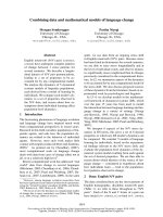
Figure 1: Formation of discontinuities
In case of x
0
<x
1
, but e.g. 0 <f

(v
0
(x

1
)) <f

(v
0
(x
0
))
14
, the characteristic
through (x
0
, 0) intersects the characteristic through (x
1
, 0) at an instant t
1
> 0,so
that at the point of intersection the solution v hastohavethevalue v
0
(x
0
) as well as
the value v
0
(x
1
) = v
0
(x
0

). Therefore, a discontinuity will occur at the instant t
1
or
even earlier. With respect to fluid dynamics, particularly shocks – discussed later on
– belong to the various types of discontinuities.
Applied to Burgers’ equation (1.16) with the initial function (1.16a), the characteristic
through a point x
0
of the x-axisisgivenby
t =2
x − x
0
2 − x
0
,
such that the discontinuity we had found at t =2 can also immediately be understood
by means of Figure 2.
If systems of conservation laws are considered instead of the scalar case, i.e.
V (x, t) ∈
m
,m∈ , ∀(x, t) ∈ Ω ,
and if only one spatial variable x occurs, a system of characteristics is defined as
follows:
Definition:
If
V (x, t)
is a solution of
(1.10)
in the case of only one space variable
x

,the
one-parameter set
x
(i)
= x
(i)
(t, χ)(χ ∈ :
set parameter
)
14
hence also v
0
(x
0
) = v
0
(x
1
)
1.2 Characteristics and Singularities 27
Figure 2: Discontinuity of the solution of the Burgers equation
of real curves defined by the ordinary differential equation
˙x = λ
i
(V (x,t)) (1.18)
for every fixed
i (i =1, ,m)
is called the set of
i–characteristics
of the partic-

ular system that belongs to
V .
Here,
λ
i
(V )(i =1, ··· ,m)
are the eigenvalues
of the Jacobian
Jf(V ).
Obviously, this definition coincides in case of m =1 with the previously presented
definition of characteristics.
Let us finally and exemplarily study the situation of a system of conservation laws if
the system is linear with constant coefficients:
∂
t
V + A ∂
x
V = 0 (1.19)
with a constant Jacobian (m, m)-matrix A. Moreover, let us assume the system to be
strictly hyperbolic.
From (1.18), the characteristics turn out to be the set of straight lines given by
x
(i)
(t)=λ
i
t + x
(i)
(0) , (i =1, ···m),
and independent of V . Hence, for every fixed i, the characteristics belonging to this
set are parallel.

If S =(s
1
, s
2
, ··· , s
m
) is the matrix whose columns consist of the eigenvectors of
the Jacobian and if Λ denotes the diagonal matrix consisting of the eigenvalues of A,
A = SΛS
−1
follows.