Fourier transforms in spectroscopy kauppinen j

Jyrki Kauppinen, Jari Partanen
Fourier Transforms in Spectroscopy
Fourier Transforms in Spectroscopy. J. Kauppinen, J. Partanen
Copyright © 2001 Wiley-VCH Verlag GmbH
ISBNs: 3-527-40289-6 (Hardcover); 3-527-60029-9 (Electronic)
Jyrki Kauppinen, Jari Partanen
Fourier Transforms
in Spectroscopy
Berlin × Weinheim × New York × Chichester
Brisbane × Singapore × Toronto
Fourier Transforms in Spectroscopy. J. Kauppinen, J. Partanen
Copyright © 2001 Wiley-VCH Verlag GmbH
ISBNs: 3-527-40289-6 (Hardcover); 3-527-60029-9 (Electronic)
Authors:
Prof. Dr. Jyrki Kauppinen Dr. Jari Partanen
Department of Applied Physics Department of Applied Physics
University of Turku University of Turku
Finland Finland
e-mail: e-mail:
This book was carefully produced. Nevertheless, authors and publisher do not warrant the
information contained therein to be free of errors. Readers are advised to keep in mind that
statements, data, illustrations, procedural details or other items may inadvertently be
inaccurate.
1st edition, 2001
with 153 figures
Library of Congress Card No.: applied for
A catalogue record for this book is available from the British Library.
Die Deutsche Bibliothek - CIP Cataloguing-in-Publication-Data
A catalogue record for this publication is available from Die Deutsche Bibliothek
ISBN 3-527-40289-6
© WILEY-VCH Verlag Berlin GmbH, Berlin (Federal Republic of Germany), 2001

Printed on acid-free paper.
All rights reserved (including those of translation in other languages). No part of this book may be
reproduced in any form - by photoprinting, microfilm, or any other means - nor transmitted or
translated into machine language without written permission from the publishers. Registered
names, trademarks, etc. used in this book, even when not specifically marked as such, are not to be
considered unprotected by law.
Printing: Strauss Offsetdruck GmbH, D-69509 Mörlenbach. Bookbinding: J. Schäffer GmbH &
Co. KG, D-67269 Grünstadt.
Printed in the Federal Republic of Germany.
WILEY-VCH Verlag Berlin GmbH
Bühringstraße 10
D-13086 Berlin
Federal Republic of Germany
Fourier Transforms in Spectroscopy. J. Kauppinen, J. Partanen
Copyright © 2001 Wiley-VCH Verlag GmbH
ISBNs: 3-527-40289-6 (Hardcover); 3-527-60029-9 (Electronic)
Preface
How much should a good spectroscopist know about Fourier transforms? How well should a
professional who uses them as a tool in his/her work understand their behavior? Our belief
is, that a profound insight of the characteristics of Fourier transforms is essential for their
successful use, as a superficial knowledge may easily lead to mistakes and misinterpretations.
But the more the professional knows about Fourier transforms, the better he/she can apply all
those versatile possibilities offered by them.
On the other hand, people who apply Fourier transforms are not, generally, mathemati-
cians. Learning unnecessary details and spending years in specializing in the heavy math-
ematics which could be connected to Fourier transforms would, for most users, be a waste
of time. We believe that there is a demand for a book which would cover understandably
those topics of the transforms which are important for the professional, but avoids going into
unnecessarily heavy mathematical details. This book is our effort to meet this demand.
We recommend this book for advanced students or, alternatively, post-graduate students

of physics, chemistry, and technical sciences. We hope that they can use this book also
later during their career as a reference volume. But the book is also targeted to experienced
professionals: we trust that they might obtain new aspects in the use of Fourier transforms by
reading it through.
Of the many applications of Fourier transforms, we have discussed Fourier transform
spectroscopy (FTS) in most depth. However, all the methods of signal and spectral processing
explained in the book can also be used in other applications, for example, in nuclear magnetic
resonance (NMR) spectroscopy, or ion cyclotron resonance (ICR) mass spectrometry.
We are heavily indebted to Dr. Pekka Saarinen for scientific consultation, for planning
problems for the book, and, finally, for writing the last chapter for us. We regard him as a
leading specialist of linear prediction in spectroscopy. We are also very grateful to Mr. Matti
Hollberg for technical consultation, and for the original preparation of most of the drawings
in this book.
Jyrki Kauppinen and Jari Partanen
Turku, Finland, 13th October 2000
Fourier Transforms in Spectroscopy. J. Kauppinen, J. Partanen
Copyright © 2001 Wiley-VCH Verlag GmbH
ISBNs: 3-527-40289-6 (Hardcover); 3-527-60029-9 (Electronic)
Contents
1Basic definitions 11
1.1 Fourier series . . . 11
1.2 Fourier transform 14
1.3 Dirac’s delta function . . . . . 17
2General properties of Fourier transforms 23
2.1 Shift theorem . . . 24
2.2 Similarity theorem . . . . . . . 25
2.3 Modulation theorem . . . . . . . . . . . . . . . . . . . . . . . . . . . . . . 26
2.4 Convolution theorem . . . . . . 26
2.5 Power theorem . . . 28
2.6 Parseval’s theorem . . . . . . 29

2.7 Derivative theorem . . . . . . 29
2.8 Correlation theorem . . . . . . 30
2.9 Autocorrelation theorem . . . . 31
3Discrete Fourier transform 35
3.1 Effect of truncation . . . . . . . 36
3.2 Effect of sampling . 39
3.3 Discrete spectrum 43
4Fast Fourier transform (FFT) 49
4.1 Basis of FFT . . . . 49
4.2 Cooley–Tukey algorithm . . . . . 54
4.3 Computation time . 56
5Other integral transforms 61
5.1 Laplace transform . . . . . . . 61
5.2 Transfer function of a linear system . . 66
5.3 z transform . 73
6Fourier transform spectroscopy (FTS) 77
6.1 Interference of light . . . . . . 77
6.2 Michelson interferometer . . . 78
6.3 Sampling and truncation in FTS 83
Fourier Transforms in Spectroscopy. J. Kauppinen, J. Partanen
Copyright © 2001 Wiley-VCH Verlag GmbH
ISBNs: 3-527-40289-6 (Hardcover); 3-527-60029-9 (Electronic)
8 0Contents
6.4 Collimated beam and extended light source . . . . . . . . . . . . . . . . . 89
6.5 Apodization . . . . . . . . . . . . . . . . . . . . . . . . . . . . . . . . . . 99
6.6 Applications of FTS . . . . . . . 100
7Nuclear magnetic resonance (NMR) spectroscopy 109
7.1 Nuclear magnetic moment in a magnetic field . . . 109
7.2 Principles of NMR spectroscopy 112
7.3 Applications of NMR spectroscopy . . . 115

8Ion cyclotron resonance (ICR) mass spectrometry 119
8.1 Conventional mass spectrometry . . . 119
8.2 ICR mass spectrometry . . . . . 121
8.3 Fourier transforms in ICR mass spectrometry 124
9Diffraction and Fourier transform 127
9.1 Fraunhofer and Fresnel diffraction . . . . . . . . . . . . . . . . . . . . . . 127
9.2 Diffraction through a narrow slit . . . . . . . . . . . . . . . . . . . . . . . 128
9.3 Diffraction through two slits . . . . . . . . . . . . . . . . . . . . . . . . . 130
9.4 Transmission grating . . . . . 132
9.5 Grating with only three orders 137
9.6 Diffraction through a rectangular aperture . . . . . . . . . . . . . . . . . . 138
9.7 Diffraction through a circular aperture . . . . . . . . . . . . . . . . . . . . 143
9.8 Diffraction through a lattice . . . . . . . . . . . . . . . . . . . . . . . . . . 144
9.9 Lens and Fourier transform . . 145
10 Uncertainty principle 155
10.1 Equivalent width . . . . . . . . . 155
10.2 Moments of a function . . . . . . . 158
10.3 Second moment . . 160
11 Processing of signal and spectrum 165
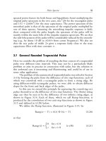
11.1 Interpolation . . . . 165
11.2 Mathematical filtering . . . . . . 170
11.3 Mathematical smoothing . . . . 180
11.4 Distortion and
(
S/N
)
enhancement in smoothing . . 184
11.5 Comparison of smoothing functions . . . . . . . . . . . . . . . . . . . . . 190
11.6 Elimination of a background . . . . . . . . . . . . . . . . . . . . . . . . . 193
11.7 Elimination of an interference pattern . . 194

11.8 Deconvolution . . . 196
12 Fourier self-deconvolution (FSD) 205
12.1 Principle of FSD . . 205
12.2 Signal-to-noise ratio in FSD . . 212
12.3 Underdeconvolution and overdeconvolution . . . . . . . . . . . . . . . . . 217
12.4 Band separation . 218
12.5 Fourier complex self-deconvolution . . . 219
9
12.6 Even-order derivatives and FSD . . 221
13 Linear prediction 229
13.1 Linear prediction and extrapolation . . . 229
13.2 Extrapolation of linear combinations of waves . . . . . . . . . . . . . . . . 230
13.3 Extrapolation of decaying waves . . . . . . . . . . . . . . . . . . . . . . . 232
13.4 Predictability condition in the spectral domain . . . . . . . . . . . . . . . . 233
13.5 Theoretical impulse response . . . . . . . . . . . . . . . . . . . . . . . . . 234
13.6 Matrix method impulse responses . . . . . . . . . . . . . . . . . . . . . . 236
13.7 Burg’s impulse response . . . . . . . . . . . . . . . . . . . . . . . . . . . 239
13.8 The q-curve . 240
13.9 Spectral line narrowing by signal extrapolation . . . . . . . . . . . . . . . 242
13.10 Imperfect impulse response . . . . . . . . . . . . . . . . . . . . . . . . . . 243
13.11 The LOMEP line narrowing method . . 248
13.12 Frequency tuning method . . . . . . . . . . . . . . . . . . . . . . . . . . . 250
13.13 Other applications . . . . . . . . 255
13.14 Summary . . 258
Answers to problems 261
Bibliography 265
Index 269
1Basic definitions
1.1 Fourier series
If a function h(t),which varies with t,satisfies the Dirichlet conditions

1. h(t) is defined from t =−∞to t =+∞and is periodic with some period T ,
2. h(t) is well-defined and single-valued (except possibly in a finite number of points) in
the interval

−
1
2
T,
1
2
T

,
3. h(t) and its derivative dh(t)/dt are continuous (except possibly in a finite number of step
discontinuities) in the interval

−
1
2
T,
1
2
T

,and
4. h(t) is absolutely integrable in the interval

−
1
2

T,
1
2
T

,thatis,
T/2

−T /2
|h(t)|dt < ∞,
then the function h(t) can be expressed as a Fourier series expansion
h(t) =
1
2
a
0
+
∞

n=1
[
a
n
cos(nω
0
t) + b
n
sin(nω
0
t)

]
=
∞

n=−∞
c
n
e
inω
0
t
, (1.1)
where














































ω
0

=
2π
T
= 2π f
0
,
a
n
=
2
T
T/2

−T /2
h(t) cos(nω
0
t) dt,
b
n
=
2
T
T/2

−T /2
h(t) sin(nω
0
t) dt,
c
n

=
1
T
T/2

−T /2
h(t)e
−inω
0
t
dt =
1
2
(a
n
− ib
n
),
c
−n
= c
∗
n
=
1
2
(a
n
+ ib
n

).
(1.2)
Fourier Transforms in Spectroscopy. J. Kauppinen, J. Partanen
Copyright © 2001 Wiley-VCH Verlag GmbH
ISBNs: 3-527-40289-6 (Hardcover); 3-527-60029-9 (Electronic)
12 1Basic definitions
f
0
is called the fundamental frequency of the system. In the Fourier series, a function h(t)
is analyzed into an infinite sum of harmonic components at multiples of the fundamental
frequency. The coefficients a
n
, b
n
and c
n
are the amplitudes of these harmonic components.
At every point where the function h(t) is continuous the Fourier series converges uni-
formly to h(t).Ifthe Fourier series is truncated, and h(t) is approximated by a sum of only
afinite number of terms of the Fourier series, then this approximation differs somewhat from
h(t).Generally, the approximation becomes better and better as more and more terms are
included.
At every point t = t
0
where the function h(t) has a step discontinuity the Fourier series
converges to the average of the limiting values of h(t) as the point is approached from above
and from below:

lim
ε→0+

h(t
0
+ ε) + lim
ε→0+
h(t
0
− ε)

2.
Around a step discontinuity, a truncated Fourier series overshoots at both sides near the
step, and oscillates around the true value of the function h(t).This oscillation behavior in the
vicinity of a point of discontinuity is called the Gibbs phenomenon.
The coefficients c
n
in Equation 1.1 are the complex amplitudes of the harmonic compo-
nents at the frequencies f
n
= nf
0
= n/T .The complex amplitudes c
n
as a function of the
corresponding frequencies f
n
constitute a discrete complex amplitude spectrum.
Example 1.1: Examine the Fourier series of the square wave shown in Figure 1.1.
Solution. Applying Equation 1.2, the square wave can be expressed as the Fourier series
h(t) =
4
π


cos(ω
0
t) −
1
3
cos(3ω
0
t) +
1
5
cos(5ω
0
t) − ···

=
4
π
∞

n=1
sin(nπ/2)
n
cos(nω
0
t).
Figure 1.1: Square wave h(t).
1.1 Fourier series 13
If this Fourier series is truncated, and the function is approximated by a finite sum, then
this approximation differs from the original square wave, especially around the points of

discontinuity. Figure 1.2 illustrates the Gibbs oscillation around the point t = t
0
of the square
wave of Figure 1.1.
The amplitude spectrum of the square wave of Figure 1.1 is shown in Figure 1.3. The
amplitude coefficients of the square wave are c
n
=
1
2
a
n
= 0,
2
π
, 0, −
2
3π
, 0,
2
5π
, 0,
Figure 1.2: The principle how the truncated Fourier series of the square wave h(t) of Fig. 1.1 oscillates
around the true value in the vicinity of the point of discontinuity t = t
0
.
Figure 1.3: Discrete amplitude spectrum of the square wave h(t) of Fig. 1.1, formed by the amplitude
coefficients c
n
. f

0
is the fundamental frequency.
14 1Basic definitions
1.2 Fourier transform
The Fourier series, Equation 1.1, can be used to analyze periodic functions of a period T and
afundamental frequency f
0
=
1
T
.Byletting the period tend to infinity and the fundamental
frequency to zero, we can obtain a generalization of the Fourier series which also is suitable
for analysis of non-periodic functions.
According to Equation 1.1,
h(t) =
∞

n=−∞
1
T
T/2

−T /2
h(t

)e
−i2π nf
0
t


dt

  
c
n
e
i12πnf
0
t
. (1.3)
We shall replace nf
0
by f ,andletT →∞and 1/T = f
0
= d f → 0. In this case,
∞

n=−∞
1
T
→
∞

−∞
d f, (1.4)
and
h(t) =
∞

−∞



∞

−∞
h(t

)e
−i2π ft

dt




 
H( f )
e
i2π ft
d f. (1.5)
We can interpret this formula as the sum of the waves H( f ) d fe
i2π ft
.
With the help of the notation H ( f ),wecan write Equation 1.5 in the compact form
h(t) =
∞

−∞
H( f )e
i2π ft

d f = {H( f )}. (1.6)
The operation
is called the Fourier transform.Fromabove,
H( f ) =
∞

−∞
h(t)e
−i2π ft
dt =
−1
{h(t)}. (1.7)
The operation
−1
is called the inverse Fourier transform.
Functions h(t) and H( f ) which are connected by Equations 1.6 and 1.7 constitute a
Fourier transform pair. Notice that even though we have used as the variables the symbols t
and f ,which often refer to time
[
s
]
and frequency
[
Hz
]
,the Fourier transform pair can be
formed for any variables, as long as the product of their dimensions is one (the dimension of
one variable is the inverse of the dimension of the other).
1.2 Fourier transform 15
In the literature, it is possible to find several, slightly differing ways to define the Fourier

integrals. They may differ in the constant coefficients in front of the integrals and in the
exponents. In this book we have chosen the definitions in Equations 1.6 and 1.7, because they
are the most convenient for our purposes. In our definition, the exponential functions inside the
integrals carry the coefficient 2π,because, in this way, we can avoid the coefficients in front
of the integrals. We have noticed that coefficients in front of Fourier integrals are a constant
source of mistakes in calculations, and, by our definition, these mistakes can be avoided. Also
the theorems of Fourier transform are essentially simpler, if this definition is chosen: in this
wayeventhey, except the derivative theorem, have no front coefficients.
The definition of the Fourier transform pair remains sensible, if a constant c is added
in front of one integral and its inverse, constant 1/c,isadded in front of the other integral.
The product of the front coefficients should equal one. We strongly encourage not to use
definitions which do not fulfill this condition. An example of this kind of definition, sometimes
encountered in literature, is obtained by setting f = ω/2π in Equations 1.6 and 1.7. We obtain
h(t) =
1
2π
∞

−∞
H(ω)e
iωt
dω = {H(ω)}, (1.8)
and
H(ω) =
∞

−∞
h(t)e
−iωt
dt =

−1
{h(t)}. (1.9)
We do not recommend these definitions, since they easily lead to difficulties.
In our definition, the exponent inside the Fourier transform
carries a positive sign,
and the exponent inside the inverse Fourier transform
−1
carries a negative sign. It is
more common to make the definition vice versa: generally the exponent inside the Fourier
transform
has a negative sign, and the exponent inside the inverse Fourier transform
−1
has a positive sign. Our book mainly discusses symmetric functions, and the Fourier transform
and the inverse Fourier transform of a symmetric function are the same. Consequently, the
choice of the sign has no scientific meaning. In our opinion, our definition is more logical,
simpler, and easier to memorize: + sign in the exponent corresponds to
and − sign in the
exponent corresponds to
−1
!
We recommend that, while reading this book, the reader forgets all other definitions and
uses only this simplest definition. In other contexts, the reader should always check, which
definition of Fourier transforms is being used.
Table 1.1 lists a few important Fourier transform pairs, which will be useful in this book,
as well as the full width at half maximum, FWHM, of these functions.
16 1Basic definitions
Table 1.1: Fourier transform pairs h(t) and H ( f ),and the FWHM of these functions.
Name FWHM
−1
, Name FWHM

of h(t)
h(t) of h(t) ⇔ of H(t ) H( f ) of H ( f )
boxcar 
2T
(t) =

1, |t|≤T,
0, |t| > T
2T sinc 2T sinc(π 2Tf)
1.2067
2T
triangular 
T
(t) =

1 −
|t|
T
, |t|≤T,
0, |t| > T
T sinc
2
T sinc
2
(π Tf)
1.7718
2T
Lorentzian
σ/π
σ

2
+ t
2
2σ exponential exp(−π 2σ |f |)
ln 2
πσ
Gaussian

α
π
exp(−αt
2
) 2

ln 2
α
Gaussian exp

−π
2
f
2
α

2
π
√
α ln 2
Dirac’s
delta δ(t −t

0
) 0 ⇒ exponential wave exp(i2π t
0
f ) —
Dirac’s
−1
delta δ(t −t
0
) 0 ⇒ exponential wave exp(−i2π t
0
f ) —
1.3 Dirac’s delta function 17
Example 1.2: Applying Fourier transforms, compute the integral
∞

0
sin( px) cos(qx)
x
dx ,
where p > 0and p = q.
Solution. Knowing that the imaginary part of e
iqx
is antisymmetric, we can write
∞

0
sin( px) cos(qx)
x
dx =
p

2
∞

−∞
sin( px)
px
e
iqx
dx =
p
2
∞

−∞
sinc(px)e
i2π
q
2π
x
dx
=
π
2
h(
q
2π
),
where the function
h(t) =
{

p
π
sinc(π
p
π
f )}.
From Table 1.1, we know that the Fourier transform of a sinc function is a boxcar function.
Consequently,
π
2
h(
q
2π
) =
π
2

p/π
(
q
2π
) =

π/2, |q| < p,
0, |q| > p.
1.3 Dirac’s delta function
Dirac’s delta function, δ(t),also called the impulse function,isaconcept which is frequently
used to describe quantities which are localized in one point. Even though real physical
quantities cannot be truly localized in exactly one point, the concept of Dirac’s delta function
is very useful.

Dirac’s delta function is defined with the following equation:
∞

−∞
F(t)δ(t − t
0
) dt = F(t
0
), (1.10)
where F(t) is an arbitrary function of t,continuous at the point t = t
0
.
By inserting the function F(t) ≡ 1inEquation 1.10, we can see that the area of Dirac’s
delta function is equal to unity, that is,
∞

−∞
δ(t −t
0
) dt = 1. (1.11)
In the usual sense, δ(t) is not really a function at all. In practice,
lim
t→t
0
δ(t −t
0
) =∞. (1.12)
At points t = t
0
either δ(t −t

0
) = 0orδ(t) oscillates with infinite frequency.
18 1Basic definitions
It can be shown that Dirac’s delta function has the following properties:



















δ(−t)
∧
= δ(t),
tδ(t)
∧
= 0,
δ(at )

∧
=
1
a
δ(t), if a > 0,
dδ(t)
dt
∧
=−
1
t
δ(t),
F(t)δ(t − t
0
)
∧
= F(t
0
)δ(t − t
0
),
(1.13)
where the correspondence relation
∧
= means that the value of the integral in Equation 1.10
remains the same whichever side of the relation is inserted in the integral.
The “shape” of Dirac’s delta function is not uniquely defined. There are infinitely many
representations of δ(t) which satisfy Equation 1.10. One of them, very useful with Fourier
transforms, is
δ(t) =

∞

−∞
e
i2πts
ds = {1}=
∞

−∞
cos(2πts) ds. (1.14)
Equivalently, we can write
δ(t) =
∞

−∞
e
−i2π ts
ds =
−1
{1}=
∞

−∞
cos(2πts) ds. (1.15)
Afew other useful representations for Dirac’s delta function are, for example,
δ(t)
∧
= lim
a→∞
sin(aπt)

πt
∧
= lim
σ →0+
σ/π
t
2
+ σ
2
∧
= lim
a→∞
a
2
e
−a|t|
∧
= lim
a→0+
1
a
√
2π
e
−t
2
/(2a
2
)
. (1.16)

Tworather simple representations are
δ(t)
∧
= lim
a→0+
f (t, a)
∧
= lim
a→0+
g(t, a), (1.17)
where f (t, a) and g(t, a) are the functions illustrated in Figure 1.4.
1.3 Dirac’s delta function 19
Figure 1.4: Tworepresentations for Dirac’s delta function: δ(t)
∧
= lim
a→0+
f (t, a)
∧
= lim
a→0+
g(t, a).
Example 1.3: Using Dirac’s delta function in the form of Equation 1.14, prove that Equa-
tion 1.6 yields Equation 1.7.
Solution. If h(t) =
∞

−∞
H( f )e
i2π ft
d f ,then

−1
{h(t)}=
∞

−∞
h(t)e
−i2π f

t
dt =
∞

−∞
∞

−∞
H( f )e
i2πt( f −f

)
d f dt
=
∞

−∞
H( f )


∞


−∞
e
i2πt( f −f

)
dt


d f
(1.14)
=
∞

−∞
H( f )δ( f − f

) d f
(1.10)
= H( f

).
Consequently,
H( f ) =
∞

−∞
h(t)e
−i2π ft
dt,
that is, Equation 1.6 ⇒ Equation1.7.

20 1Basic definitions
Problems
1. Show that the Fourier transform and the inverse Fourier transform
−1
of a symmetric
function are the same. Also show that these Fourier transforms are symmetric.
2. Compute
{ {h(t)}} and
−1
{
−1
{h(t)}}.
3. Derive the Fourier transforms of the Gaussian curve, i.e.,


α
π
exp

−α f
2


and
−1


α
π
exp


−α f
2


,
where α>0.
4. Derive the Fourier transform of the Lorentzian function L( f ) =
σ/π
f
2
+ σ
2
, σ>0.
(Function L( f ) is symmetric, and hence
and
−1
are the same.)
Hint: Use the following integral from mathematical tables:
∞

0
cos(Cx)
x
2
+ a
2
dx =
π
2a

e
−Ca
,
where C, a > 0.
5. Applying Fourier transforms, compute the integral I =
T

−T
(T −|t|) cos[2π f
0
(T −t)]dt.
6. Let us denote 
2T

(t) the boxcar function of the width 2T

,stretching from −T

to T

,
and of one unit height. The sum of N boxcar functions
1
N

1
N
2T
(t),
1

N

2
N
2T
(t),
1
N

3
N
2T
(t), ,
1
N

2T
(t)
is a one-unit high step-pyramidal function. In the limit N →∞this pyramidal function
approaches a one-unit high triangular function 
T
(t).Determine the inverse Fourier
transform of the pyramidal function, and find the inverse Fourier transform of 
T
(t) by
letting N →∞.
Hint: You may need the trigonometric identity
sin α + sin(2α) +···+sin(N α) =
sin


1
2
(N +1)α

sin

1
2
N α

sin(α/2)
.
7. Show that the function
δ(t) =
∞

−∞
e
i2π ft
d f
satisfies the definition of Dirac’s delta function by using the Fourier’s integral theorem
−1
{F }=F.
Problems 21
8. Show that the function f (t) = lim
σ →0
σ/π
t
2
+ σ

2
satisfies the definition of Dirac’s delta
function.
9. Let us define the step function u(t) as
u(t) =

0, t < 0,
1, t ≥ 0.
Show that the choice δ(t − t
0
) =
d
dt
0
u(t
0
− t) satisfies the condition of Dirac’s delta
function.
Hint: You can change the order of differentiation and integration.
10. Compute the integral
ε

−ε
δ(t) dt,whereε>0, by inserting δ(t) =
∞

−∞
e
±i2π ft
d f in it.

11. What are the Fourier transforms (both
and
−1
)ofthe following functions? Let us
assume that f
0
> 0.
(a) δ( f ) (Dirac’s delta peak in the origin);
(b) δ( f − f
0
) (Dirac’s delta peak at f
0
);
(c) δ( f − f
0
) + δ( f + f
0
) (Dirac’s delta peaks at f
0
and − f
0
);
(d) δ( f − f
0
) −δ( f + f
0
) (Dirac’s delta peak at f
0
and negative Dirac’s delta peak at
− f

0
).
2General properties of Fourier transforms
The general definitions of the Fourier transform and the inverse Fourier transform
−1
are
h(t) =
∞

−∞
H( f )e
i2π ft
d f = {H( f )}, (2.1)
H( f ) =
∞

−∞
h(t)e
−i2π ft
dt =
−1
{h(t)}. (2.2)
H( f ) is called the spectrum and h(t) is the signal.The inverse Fourier transform operator
−1
generates the spectrum from a signal, and the Fourier transform operator restores the
signal from a spectrum. A single point in the spectrum corresponds to a single exponential
wave in the signal, and vice versa. The signal is often defined in the time domain (t-domain),
and the spectrum in the frequency domain ( f -domain), as above.
Usually, the signal h(t) is real. The spectrum H ( f ) can still be complex, because
H( f ) =

∞

−∞
h(t)e
−i2π ft
dt =
∞

−∞
h(t) cos(2π ft) dt − i
∞

−∞
h(t) sin(2π ft) dt
=
cos
{h(t)}−i
sin
{h(t)}=|H( f )|e
iθ(f )
. (2.3)
cos
{h(t)} and
sin
{h(t)} are called the cosine transform and the sine transform,respectively,
of h(t).
|H( f )|=

[
cos

{h(t)}
]
2
+
[
sin
{h(t)}
]
2
(2.4)
is the amplitude spectrum and
θ( f ) =−arctan
sin
{h(t)}
cos
{h(t)}
(2.5)
is the phase spectrum. (Equation 2.5 is valid only when −π/2 ≤ θ ≤ π/2.) The amplitude
spectrum and the phase spectrum are illustrated in Figure 2.1. The inverse Fourier transform
and the Fourier transform can be expressed with the help of the cosine transform and the sine
transform as
−1
{h(t)}=
cos
{h(t)}−i
sin
{h(t)} (2.6)
Fourier Transforms in Spectroscopy. J. Kauppinen, J. Partanen
Copyright © 2001 Wiley-VCH Verlag GmbH
ISBNs: 3-527-40289-6 (Hardcover); 3-527-60029-9 (Electronic)

24 2General properties of Fourier transforms
and
{H( f )}=
cos
{H( f )}+i
sin
{H( f )}. (2.7)
Often, i
sin
{H( f )} equals zero.
Figure 2.1: The amplitude spectrum |H( f )| and the phase spectrum θ(f ).
In the following, a collection of theorems of Fourier analysis is presented. They contain
the most important characteristic features of Fourier transforms.
2.1 Shift theorem
Let us consider how a shift ± f
0
of the frequency of a spectrum H ( f ) affects the corresponding
signal h(t),which is the Fourier transform of the spectrum. We can find this by making a
change of variables in the Fourier integral:
{H( f ± f
0
)}=
∞

−∞
H( f ± f
0
)e
i2π ft
d f

g=f ±f
0
dg=d f
=
∞

−∞
H(g)e
i2π(g∓f
0
)t
dg = e
∓i2π f
0
t
∞

−∞
H(g)e
i2πgt
dg
= h(t)e
±i2π f
0
t
.
Likewise, we can obtain the effect of a shift ±t
0
of the position of the signal h(t) on the
spectrum H( f ),which is the inverse Fourier transform of the signal.

These results are called the shift theorem.The theorem states how the shift in the position
of a function affects its transform. If H ( f ) =
−1
{h(t)},and both t
0
and f
0
are constants,
then
{H( f ± f
0
)}= {H ( f )}e
∓i2π f
0
t
= h(t)e
∓i2π f
0
t
,
−1
{h(t ± t
0
)}=
−1
{h(t)}e
±i2π ft
0
= H( f )e
±i2π ft

0
.
(2.8)
2.2 Similarity theorem 25
This means that the Fourier transform of a shifted function is the Fourier transform of the
unshifted function multiplied by an exponential wave or phase factor. The same holds true for
the inverse Fourier transform.
If a function is shifted away from the origin, its transform begins to oscillate at the
frequency given by the shift. A shift in the location of a function in one domain corresponds
to multiplication by a wave in the other domain.
2.2 Similarity theorem
Let us next examine multiplication of the frequency of a spectrum by a positive real constant a.
We shall take the Fourier transform, and apply the change of variables:
{H(af)}=
∞

−∞
H(af)e
i2π ft
d f
g=af
dg=ad f
=
∞

−∞
1
a
H(g)e
i2πgt/a

dg
=
1
a
h(t/a).
The inverse Fourier transform of a signal can be examined similarly.
We obtain the results that if H( f ) =
−1
{h(t)},anda is a positive real constant, then
{H(af)}=
1
a
h(t/a),
(2.9)
and
−1
{h(at )}=
1
a
H( f/a).
(2.10)
These statements are called the similarity theorem,orthescaling theorem,ofFourier trans-
forms. The theorem tells that a contraction of the coordinates in one domain leads to a
corresponding stretch of the coordinates in the other domain.
If a function is made to decay faster (a > 1), keeping the height constant, then the Fourier
transform of the function becomes wider, but lower in height. If a function is made to decay
slower (0 < a < 1), its Fourier transform becomes narrower, but taller. The same applies to
the inverse Fourier transform
−1
.

26 2General properties of Fourier transforms
2.3 Modulation theorem
The modulation theorem explains the behavior of the Fourier transform when a function is
modulated by multiplying it by a harmonic function. A straightforward computation gives
that
{H( f ) cos(2πt
0
f )}=
∞

−∞
H( f ) cos(2πt
0
f )e
i2π ft
d f
=
∞

−∞
H( f )
e
i2πt
0
f
+ e
−i2π t
0
f
2

e
i2π ft
d f
=
1
2
∞

−∞
H( f )e
i2π(t+t
0
) f
d f +
1
2
∞

−∞
H( f )e
i2π(t−t
0
) f
d f
=
1
2
h(t + t
0
) +

1
2
h(t − t
0
).
Asimilar result can be obtained for the inverse Fourier transform.
Consequently, we obtain that if H( f ) =
−1
{h(t)},andt
0
and f
0
are real constants, then
{H( f ) cos(2πt
0
f )}=
1
2
h(t + t
0
) +
1
2
h(t − t
0
), (2.11)
and
−1
{h(t) cos(2π f
0

t)}=
1
2
H( f + f
0
) +
1
2
H( f − f
0
). (2.12)
These results are the modulation theorem. The Fourier transform of a function multiplied by
cos(2πt
0
f ) is the average of two Fourier transforms of the original function, one shifted in the
negative direction by the amount t
0
,and the other in the positive direction by the amount t
0
.
The inverse Fourier transform is affected by harmonic modulation in a similar way.
2.4 Convolution theorem
The convolution of functions g(t) and h(t) is defined as
g(t) ∗ h(t) =
∞

−∞
g(u)h(t − u) du. (2.13)
This convolution integral is a function which varies with t.Itcan be thought as the area of the
product of g(u) and h(t − u),varying with t.One of the two functions is folded backwards:

h(−u) is the mirror image of h(u),reflected about the origin. This is illustrated in Figure 2.2.
2.4 Convolution theorem 27
Figure 2.2: The principle of convolution. Convolution of the two functions g(t) and h(t) (upper curves)
is the area of the product g(u)h(t − u) (the hatched area inside the lowest curve), as a function of the
shift t of h (−u).
The function g can be thought to be an object function, which is convolved by the other,
convolving function h.The convolving function is normally a peak-shaped function, and the
effect of the convolution is to smear the object function. If also the object function is peak-
shaped, then the convolution broadens it.
Convolution is always broader than the broadest of the two functions which are convolved.
Convolution is also always smoother than the smoothest of the two functions. Convolution
with Dirac’s delta function is a special borderline case:
δ(t) ∗ f (t) = f (t), (2.14)
and thus convolution with Dirac’s delta function is as broad and as smooth as the second
function.
28 2General properties of Fourier transforms
Convolution can be shown to have the following properties:



h ∗ g = g ∗ h (commutative),
h ∗ (g ∗k) = (h ∗ g) ∗ k (associative),
h ∗ (g +k) = (h ∗ g) + (h ∗ k) (distributive).
(2.15)
Let us examine the Fourier transform and the inverse Fourier transform of a product of two
functions. If H( f ) =
−1
{h(t)},andG( f ) =
−1
{g(t)},then it is can be shown (Problem 5)

that
{H( f )G( f )}= {H( f )}∗ {G( f )}=h(t) ∗ g(t),
−1
{h(t) ∗ g(t)}=
−1
{h(t)}
−1
{g(t)}=H ( f )G( f )
(2.16)
and
−1
{h(t)g(t)}=H ( f ) ∗ G( f ),
{H( f ) ∗ G( f )}=h(t)g(t).
(2.17)
These equations are the convolution theorem of Fourier transforms. They can be verified
either by a change of variables of integration or by applying Dirac’s delta function. The
convolution theorem states that convolution in one domain corresponds to multiplication in
the other domain.
The Fourier transform of the product of two functions is the convolution of the two
individual Fourier transforms of the two functions. The same holds true for the inverse Fourier
transform: the inverse Fourier transform of the product of two functions is the convolution of
the individual inverse Fourier transforms.
On the other hand, the Fourier transform of the convolution of two functions is the product
of the two individual Fourier transforms. And the inverse Fourier transform of the convolution
of two functions is the product of the two individual inverse Fourier transforms.
2.5 Power theorem
The complex conjugate u*ofacomplex number u is obtained by changing the sign of its
imaginary part, that is, by replacing i by −i.
If h(t) and H( f ),andg(t) and G( f ) are Fourier transform pairs, then
∞


−∞
h(t)g
∗
(t) dt =
∞

−∞
∞

−∞

H( f )e
i2π ft
d f

g
∗
(t) dt
=
∞

−∞
H( f )


∞

−∞
g(t)e

−i2π ft
dt


∗
d f
=
∞

−∞
H( f )G
∗
( f ) d f.
2.6 Parseval’s theorem 29
This result,
∞

−∞
h(t)g
∗
(t) dt =
∞

−∞
H( f )G
∗
( f ) d f, (2.18)
is called the power theorem of Fourier transforms: the overall integral of the product of a
function and the complex conjugate of a second function equals the overall integral of the
product of the transform of the function and the complex conjugate of the transform of the

second function.
2.6 Parseval’s theorem
The Parseval’s theorem can be deduced from the power theorem (Equation 2.18) by choosing
that h = g.Weobtain that
∞

−∞
|h(t)|
2
dt =
∞

−∞
|H( f )|
2
d f. (2.19)
The area under the squared absolute value of a function is the same as the area under the
squared absolute value of the Fourier transform of the function.
2.7 Derivative theorem
The derivative theorem states the form of the Fourier transform of the derivative of a function.
Differentiating, with respect to t, both sides of equation
h(t) =
{H( f )}=
∞

−∞
e
i2π ft
H( f ) d f, (2.20)
we obtain that

dh(t)
dt
= h
(1)
(t) =
∞

−∞
(i2π f )e
i2π ft
H( f ) d f. (2.21)
Repetition of this operation k times yields
d
k
h(t)
dt
k
= h
(k)
(t) =
∞

−∞
(i2π f )
k
e
i2π ft
H( f ) d f. (2.22)