conduction model of metal oxide gas sensors

Journal of Electroceramics, 7, 143–167, 2001
C

2002 Kluwer Academic Publishers. Manufactured in The Netherlands.
Feature Article
Conduction Model of Metal Oxide Gas Sensors
NICOLAE BARSAN & UDO WEIMAR
Institute of Physical and Theoretical Chemistry, University of Tuebingen, Auf der Morgenstelle 8, 72076 T
¨
ubingen, Germany
Submitted August 14, 2001; Revised October 31, 2001; Accepted November 7, 2001
Abstract. Tin dioxide is a widely used sensitive material for gas sensors. Many research and development groups
in academia and industry are contributing to the increase of (basic) knowledge/(applied) know-how. However, from
a systematic point of view the knowledge gaining process seems not to be coherent. One reason is the lack of a
general applicable model which combines the basic principles with measurable sensor parameters.
The approach in the presented work is to provide a frame model that deals with all contributions involved in
conduction within a real world sensor. For doing so, one starts with identifying the different building blocks of a
sensor. Afterwards their main inputs are analyzed in combination with the gas reaction involved in sensing. At the
end, the contributions are summarized together with their interactions.
The work presented here is one step towards a general applicable model for real world gas sensors.
Keywords: metal oxide, gas sensors, conduction model
1. Introduction
Metal oxides in general and SnO
2
, in particular, have
attracted the attention of many users and scientists
interested in gas sensing under atmospheric condi-
tions. SnO
2
sensors are the best-understood prototype
of oxide-based gas sensors. Nevertheless, highly spe-

cific and sensitive SnO
2
sensors are not yet available.
It is well known that sensor selectivity can be fine-
tuned over a wide range by varying the SnO
2
crys-
tal structure and morphology, dopants, contact geome-
tries, operation temperature or mode of operation, etc.
In addition, practical sensor systems may contain a
combination of a filter (like charcoal) in front of the
SnO
2
semiconductor sensor to avoid major impact
from unwanted gases (e.g. low concentrations of or-
ganic volatiles which influence CO detection). The
understanding of real sensor signals as they are mea-
sured in practical application is hence quite difficult.
It may even be necessary to separate filter and sen-
sor influences for an unequivocal modelling of sensor
responses.
In spite of extensive world wide activities in the re-
search and development of these sensors, our basic sci-
entific understanding of practically usefulgassensorsis
very poor. This results from the fact that three different
approaches are generally chosen by three different
kinds of experts. Our present understanding is hence
based on different models
r
The first approach is chosen by the users of gas sen-

sors, who test the phenomenological parameters of
available sensors in view of a minimum parame-
ter set to describe their selectivity, sensitivity, and
stability.
r
The second approach is chosen by the developers,
who empirically optimise sensor technologies by
optimising the preparation of sensor materials, test
structures, ageing procedures, filter materials, mod-
ulation conditions during sensor operation, etc. for
different applications.
r
The third approach is chosen by basic research sci-
entists, who attempt to identify the atomistic pro-
cesses of gas sensing. They apply spectroscopies
in addition to the phenomenological techniques of
sensor characterisation (such as conductivity mea-
surements), perform quantum mechanical calcula-
tions, determine simplified models of sensor oper-
ation, and aim at the subsequent understanding of
thermodynamic or kinetic aspects of sensing mecha-
nisms on the molecular scale. This is usually done on
144 Barsan and Weimar
well-defined model systems for well-defined gas ex-
posures. Consequently this leads to the well-known
structural and pressure gaps between the ideal and
the real world of surface science.
The present paper aims to bridge the gap between
basic and applied research by providing a model de-
scription of phenomena involved in the detection pro-

cess. The models are sensor focussed but are using,
to the greatest possible extent, the basic research
approach.
The use of the output of these models enables a more
specific design of real world sensors.
2. Overview: Contribution of Different
Sensor Parts in the Sensing Process
and Subsequent Transduction
A sensor element normally comprises the following
parts:
r
Sensitive layer deposited over a
r
Substrate provided with
r
Electrodes for the measurement of the electrical
characteristics. The device is generally heated by its
own
r
Heater; this one is separated from the sensing
layer and the electrodes by an electrical insulating
layer.
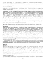
Fig. 1. Schematic layout of a typical resistive gas sensor. The sensitive metal oxide layer is deposited over the metal electrodes onto the substrate.
In the case of compact layers, the gas cannot penetrate into the sensitive layer and the gas interaction is only taking place at the geometric
surface. In the case of porous layers the gas penetrates into the sensitive layer down to the substrate. The gas interaction can therefore take place
at the surface of individual grains, at grain-grain boundaries and at the interface between grains and electrodes and grains and substrates.
Generally the conductance or the resistance of the sen-
sor is monitored as a function of the concentration of
the target gases. Additionally the performance of the
sensor depends on the

r
Measurement parameters, such as sensitive layer po-
larisation or temperature, which are controlled by
using different electronic circuits.
The elementary reaction steps of gas sensing will be
transduced into electrical signals measured by appro-
priate electrode structures. The sensing itself can take
place at different sites of the structure depending on the
morphology. They will play different roles, according
to the sensing layer morphology. An overview is given
in Fig. 1.
A simple distinction can be made between:
r
compact layers; the interaction with gases takes
place only at the geometric surface (Fig. 2, such lay-
ers are obtained with most of the techniques used for
thin film deposition) and
r
porous layers; the volume of the layer is also ac-
cessible to the gases and in this case the active sur-
face is much higher than the geometric one (Fig. 3,
such layers are characteristic to thick film tech-
niques and RGTO (Rheotaxial Growth and T hermal
Oxidation) [1]).
For compact layers, there are at least two possibilities:
completely or partly deploted layers, depending on the
ratio between layer thickness and Debye length λ
D
.
Conduction Model of Metal Oxide Gas Sensors 145

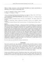
Fig. 2. Schematic representation of a compact sensing layer with geometry and energy band representations; z
0
is the thickness of the depleted
surface layer; z
g
is the layer thickness and qV
s
the band bending. a) represents a partly depleted compact layer (“thicker”), b) represents a
completely depleted layer (“thinner”). For details, see text and [17].
Fig. 3. Schematic representation of a porous sensing layer with
geometry and energy band. λ
D
Debye length, x
g
grain size. For
details, see text and [17].
For partlydepleted layers, when surface reactions do
not influence the conduction in the entire layer (z
g
> z
0
see Fig. 2), the conduction process takes place in the
bulk region (of thickness z
g
− z
0
, much more con-
ductive that the surface depleted layer). Formally two
resistances occur in parallel, one influenced by surface
reactions and the other not; the conduction is parallel

to the surface, and this explains the limited sensitivity.
Such a case is generally treated as a conductive layer
with a reaction-dependent thickness. For the case of
completely depleted layers in the absence of reducing
gases, it is possible that exposure to reducing gases
acts as a switch to the partly depleted layer case (due
to the injection of additional free charge carriers). It
is also possible that exposure to oxidizing gases acts
as a switch between partly depleted and completely
depleted layer cases.
For porous layers the situation may be complicated
further by the presence of necks between grains (Fig. 5).
It may be possible to have all three types of contribu-
tion presented in Fig. 4 in a porous layer: surface/bulk
(for large enough necks z
n
> z
0
, Fig. 5), grain bound-
ary (for large grains not sintered together), and flat
bands (for small grains and small necks). Of course,
what was mentioned for compact layers, i.e. the pos-
sible switching role of reducing gases, is valid also
146 Barsan and Weimar
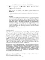
Fig. 4. Different conduction mechanisms and changes upon O
2
and CO exposure to a sensing layer in overview: This survey shows geometries,
electronic band pictures and equivalent circuits. E
C
minimum of the conduction band, E

V
maximum of the valence band, E
F
Fermi level, and
λ
D
Debye length. For details, see text and [18].
Fig. 5. Schematic representation of a porous sensing layer with geometry and surface energy band-case with necks between grains. z
n
is the
neck diameter; z
0
is the thickness of the depletion layer. a) represents the case of only partly depleted necks whereas b) represents large grains
where the neck contact is completely depleted. For details, see text and [17].
for porous layers. For small grains and narrow necks,
when the mean free path of free charge carriers be-
comes comparable with the dimension of the grains,
a surface influence on mobility should be taken into
consideration. This happens because the number of
collisions experienced by the free charge carriers in the
bulk of the grain becomes comparable with the number
of surface collisions; the latter may be influenced by
Conduction Model of Metal Oxide Gas Sensors 147
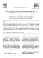
Fig. 6. Schematic representation of compact and porous sensing layers with geometry and energetic bands, which shows the possible influence
of electrode-sensing layers contacts. R
C
is the resistance of the electrode-SnO
2
contact, R
l1

is the resistance of the depleted region of the compact
layer, R
l2
is the resistance of the bulk region of the compact layer, R
1
is the equivalent series resistance of R
l1
and R
C
, R
2
is the equivalent
series resistance of R
l2
and R
C
, R
gi
is the average intergrain resistance in the case of porous layer, E
b
is the minimum of the conduction band
in the bulk, qV
S
is the band bending associated with surface phenomena on the layer, and qV
C
also contains the band bending induced at the
electrode-SnO
2
contact.
adsorbed species acting as additional scattering centres

(see discussion in [2]).
Figure 6 illustrates the way in which the metal-
semiconductor junction, built at electrodesensitive
layer interfaces, influences the overall conduction pro-
cess. For compact layers they appear as a contact re-
sistance (R
C
) in series with the resistance of the SnO
2
layer. For partly depleted layers, R
C
could be dominant,
and the reactions taking place at the three-phase bound-
ary, electrode-SnO
2
-atmosphere, control the sensing
properties.
In porous layers the influence of R
C
may be min-
imized due to the fact that it will be connected in
series with a large number of resistances, typically
thousands, which may have comparable values (R
gi
in
Fig. 6). Transmission line measurements (TLM) per-
formed with thick SnO
2
layers exposed to CO and
NO

2
did not result in values of R
C
clearly distinguish-
able from the noise [3], while in the case of dense
thin films the existence of R
C
was proved [4]. Again,
the relative importance played by different terms may
be influenced by the presence of reducing gases due
to the fact that one can expect different effects for
grain-grain interfaces when compared with electrode-
grain interfaces.
3. Influence of Gas Reaction on the Surface
Concentration of Free Charge Carriers
In the following, different contributions to the charge
carrier concentration, n
S
, in the depletion layer at the
surface will be described.
3.1. Oxygen
At temperatures between 100 and 500
◦
C the interaction
with atmospheric oxygen leads to its ionosorption in
molecular (O
−
2
) and atomic (O
−

,O
−−
) forms (Fig. 7).
It is proved by TPD, FTIR, and ESR that below 150
◦
C
the molecular form dominates and above this tempera-
ture the ionic species dominate. The presence of these
species leads to the formation of a depletion layer at the
surface of tin oxide. We will assume that in the cases
we are examining, the surface coverage is dominated
by one species. The dominating species are depending
on temperature and, probably, on surface dopants.
The equation describing the oxygen chemisorption
can be written as:
β
2
O
gas
2
+ α · e
−
+ S


O
−α
β S
(1)
148 Barsan and Weimar

Fig. 7. Literature survey of oxygen species detected at different temperatures at SnO
2
surfaces with IR (infrared analysis), TPD (temperature
programmed desorption), EPR (electron paramagnetic resonance). For details, see listed references.
where
O
gas
2
is an oxygen molecule in the ambient atmosphere;
e
−
is an electron, which can reach the surface that
means it has enough energy to overcome the electric
field resulting from the negative charging of the sur-
face. Their concentration is denoted n
S
; n
S
= [e
−
];
S is an unoccupied chemisorption site for oxygen–
surface oxygen vacancies and other surface defects are
generally considered candidates;
O
−α
β S
is a chemisorbed oxygen species
with:
α = 1 for singly ionised forms

α = 2 for doubly ionised form.
β = 1 for atomic forms
β = 2 for molecular form
The chemisorption of oxygen is a process that has two
parts: an electronic one and a chemical one. This fol-
lows from the fact that the adsorption is produced by
the capture of an electron at a surface state, but the sur-
face state doesn’t exist in the absence of the adsorbed
atom/molecule. This fact indicates that at the begin-
ning of the adsorption, the limiting factor is chemical,
the activation energy for adsorption /dissociation, due
to the unlimited availability of free electrons in the ab-
sence of band bending. After the building of the surface
charge, a strong limitation is coming from the potential
barrier that has to be overcome by the electrons in
order to reach the surface. Desorption is controlled,
from the very beginning, by both electronic and chem-
ical parts; the activation energy is not changed during
the process if the coverage is not high enough to pro-
vide interaction between the chemisorbed species [5].
The activation energies for adsorption and desorption
are included in the reaction constants, k
ads
and k
des
.
From Eq. (1) we can deduce using the mass action
law:
k
ads

· [S] · n
α
S
· p
β/2
O
2
= k
des
·

O
−α
β S

(2)
[S
t
] being the total concentration of available surface
sites for oxygen adsorption, occupied or unoccupied.
By defining the surface coverage θ with chemisorbed
oxygen as:
θ =

O
−α
β S

[S
t

]
(3)
and using the conservation of surface sites:
[S] +

O
−α
β S

= [S
t
] (4)
we can write:
(1 − θ) · k
ads
· n
α
S
· p
β/2
O
2
= k
des
· θ (5)
Conduction Model of Metal Oxide Gas Sensors 149
Equation (5) is giving a relationship between the
surface coverage with ionosorbed oxygen and the
concentration of electrons with enough energy to reach
the surface. If hopping of electrons from one grain to

another controls the electrical conduction in the layer,
this electron concentration is the one that is partici-
pating in conduction. Equation (5) is not enough for
finding the relationship between n
S
and the concen-
tration of oxygen in the gaseous phase, p
O
2
, due to
the fact that the surface coverage and n
S
are related.
We need an additional equation and we can use the
electroneutrality condition combined with the Poisson
equation.
The electroneutrality equation in the Schottky ap-
proximation states that the charge in the depletion layer
is equal to the charge captured at the surface.
We will consider that we are at temperatures high
enough to have all donors ionised (concentration of
ionised donors equals the bulk electron density n
b
). If
one assumes the Schottky approximation to be valid,
we will have all the electrons from the depletion layer
captured on surface levels.
The following section describes how one obtains
the second relation between θ and n
S

(the first relation
is given in Eq. (5)). The results are valid also in the
case where θ is influenced by the presence of addi-
tional gases. An example for CO will be provided in
Section 3.3.
One can distinguish between two limiting cases:
Case 1. Grains/crystallites large enough to have a
bulk region unaffected by surface phenomena (d 
λ
D
; see 3.1.1)
Case 2. Grains/crystallites smaller than or compara-
ble to λ
D
(d ≤ λ
D
; see 3.1.2)
3.1.1. Large grains. The situation is described by
Fig. 8; for large grains, one generally treats the situation
in a planar and semi-infinite manner. qV
S
is the band
bending, z
0
denotes the depth of the depleted region
and A the covered area.
In the first case (large grains), we can write the
electroneutrality (6) and the Poisson equations (7) for
energy (E) as:
α · θ · [S

t
] · A = n
b
· z
0
· A = Q
SS
(6)
d
2
E(z)
dz
2
=
q
2
· n
b
ε · ε
0
(7)
Fig. 8. Band bending after chemisorption of charged species (here
ionosorption of oxygen on E
SS
levels).  denotes the work function,
χ is the electron affinity, and µ the electrochemical potential.
the boundary conditions for the Poisson equation are
dE(z)
dz





z=z
0
= 0 (8)
E(z)|
z=z
0
= E
C
(9)
one obtains from the Poisson equation:
E(z) = E
C
+
q
2
· n
b
2 · ε · ε
0
· (z − z
0
)
2
(10)
which results in the general dependence of band bend-
ing, given that V = E/q
V (z) =

q · n
b
2 · ε · ε
0
· (z − z
0
)
2
(11)
and for the surface band bending
V
S
=
q · n
b
2 · ε · ε
0
· z
2
0
(12)
By combining Eqs. (6) and (12) and using the following
relation 13 between V
S
and n
S
n
s
= n
b

exp

−
qV
s
k
B
T

(13)
150 Barsan and Weimar
one obtains
θ =

2 · ε · ε
0
· n
b
· k
B
· T
α
2
· [S
t
]
2
· q
2
· ln

n
b
n
S
(14)
which together with Eq. (5) allows the determination
of n
S
and θ as a function of partial pressures (p
O
2
),
temperature T , ionisation and chemical state of oxygen
α, β, reaction constants k
ads
, k
des
, material constants ε,
n
b
,[S
t
] and fundamental constants, k
B
, ε
0
. The latter
relation can, for example be solved numerically or by
using different approximations.
3.1.2. Small grains. In the second case (small

grains) it is also important to evaluate the band bend-
ing between the surface and the centre of the grain. The
following discussion is originally given in [2]:
The calculations assume a conduction taking place
in cylindrical filaments (with radius R) obtained by the
sintering of small grains. Using this assumption, one
can write the Poisson equation in cylindrical coordi-
nates directly for energy E using the Schottky approx-
imation. For the given geometry, the radial part of the
Poisson equation is:

1
r
d
dr
+
d
2
dr
2

E(r) =
q
2
n
b
εε
0
(15)
The boundary conditions are:

E(r)|
r=0
= E
0
(16)
dE(r)
dr




r=0
= 0 (17)
Using Eqs. (15)–(17) one obtains for E = E(R) −
E
0
:
E =
q
2
n
b
4εε
0
R
2
(18)
or by using the formula of the Debye length obtained
in the Schottky approximation
λ

D
=

εε
0
k
B
T
q
2
n
b
(19)
one obtains
E ∼ k
B
· T ·

R
2 · λ
D

. (20)
Table 1. Bulk and surface parameters of influence for SnO
2
single
crystals. n
b
is the concentration of free charge carriers (electrons),
µ

b
is their Hall mobility, λ
D
is the Debye length, and λ is the mean
free path of free charge carriers (electrons).
T (K) 400 500 600 700
n
b
(10
19
) 1 11 58 260
µ
b
(10
−4
m
2
/(Vs)) 178 87 49 31
λ
D
(nm) 129 43 21 11
λ (nm) 1.96 1.07 0.66 0.45
E /(k
B
T )|
(R=50 nm)
0.34 0.77 1.08 1.49
If E is comparable with the thermal energy, this
leads to a homogeneous electron concentration in the
grain and in turn to the flat band case. One can show

that, using data available in the literature (see [2] and
Table 1), for grain sizes lower than 50 nm, complete
grain depletion and a flat band condition can be ac-
cepted almost for all relevant temperatures (excluding
e.g. 700 K since the value of E is larger than k
B
T ).
The electroneutrality condition now takes the form
(in flat band condition)
α · θ · [S
t
] · A + n
S
· V = n
b
· V (21)
where n
S
is now the homogenous concentration of elec-
trons throughout the whole tin oxide crystallites as il-
lustrated in Fig. 4.
Assuming that the cylinder length is L, having in
mind the surface A of a cylinder as
A = 2 · π · R · (R + L) (22)
and the volume V as
V = π · R
2
· L (23)
and combining Eqs. (21)–(23)
θ =

n
b
· R
2 · α · [S
t
] ·

1 +
R
L

·

1 −
n
S
n
b

(24)
With the approximation of R/L close to zero one
obtains
θ =
n
b
· R
2 · α · [S
t
]
·


1 −
n
S
n
b

(25)
Conduction Model of Metal Oxide Gas Sensors 151
This together with Eq. (5) allows the determination of
n
S
and θ as a function of only partial pressures ( p
O
2
),
temperature T , ionisation and chemical state of oxygen
α, β, reaction constants k
ads
, k
des
, material constants n
b
,
[S
t
] and fundamental constant k
B
. The latter relation
can be, for example, solved numerically or by using

different approximations.
3.2. Water Vapour
At temperatures between 100 and 500
◦
C, the interac-
tion with water vapour leads to molecular water and
hydroxyl groups adsorption (Fig. 9). Water molecules
can be adsorbed by physisorption or hydrogen bond-
ing. TPD and IR studies show that at temperatures
above 200
◦
C, molecular water is no more present at
the surface. Hydroxyl groups can appear due to an
acid/base reaction with the OH sharing its electronic
pair with the Lewis acid site (Sn) and leaving the hy-
drogen atom ready for reaction maybe with the lattice
oxygen, (Lewis base), or with adsorbed oxygen. IR
studies are indicating the presence of hydroxyl groups
bound to Sn atoms.
There are three types of mechanisms explaining
the experimentally proven increase of surface con-
ductivity in the presence of water vapour. Two, direct
Fig. 9. Literature survey of water-related species formed at different temperatures at SnO
2
surfaces. For details, see listed references.
mechanisms are proposed by Heiland and Kohl [6] and
the third, indirect, is suggested by Morrison and by
Henrich and Cox [5, 7].
The first mechanism of Heiland and Kohl attributes
the role of electron donor to the ‘rooted’ OH group, the

one including lattice oxygen. The equation proposed
is:
H
2
O
gas
+ Sn
Sn
+ O
O


(Sn
+
Sn
− OH
−
) + (OH)
+
O
+ e
−
(26)
Where (Sn
+
Sn
− OH
−
) is denominated as an isolated
hydroxyl or OH group and (OH)

+
O
is the rooted one. In
the upper equation, the latter is already ionised.
The reaction implies the homolytic dissociation of
water and the reaction of the neutral H atom with the
lattice oxygen. The latter is normally in the lattice fix-
ing two electrons consequently being in the 2-state.
The built up rooted OH group, having a lower electron
affinity and consequently can get ionised and become
a donor (with the injection of an electron in the con-
duction band).
The second mechanism takes into account the pos-
sibility of the reaction between the hydrogen atom and
the lattice oxygen and the binding of the resulting hy-
droxyl group to the Sn atom. The resulting oxygen
152 Barsan and Weimar
vacancy will produce, by ionisation, the additional elec-
trons. The equation proposed by Heiland and Kohl [6]
is:
H
2
O
gas
+ 2 · Sn
sn
+ O
O



2 · (Sn
+
Sn
− OH
−
) + V
++
O
+ 2 · e
−
(27)
Morrison, as well as Henrich and Cox [5, 7], consider an
indirect effect more probable. This effect could be the
interaction between either the hydroxyl group or the
hydrogen atom originating from the water molecule
with an acid or basic group, which are also acceptor
surface states. Their electronic affinity could change
after the interaction. It could also be the influence of
the co-adsorption of water on the adsorption of an-
other adsorbate, which could be an electron acceptor.
Henrich and Cox suggested that the pre-adsorbed oxy-
gen could be displaced by water adsorption. In any of
these mechanisms, the particular state of the surface has
a major role, due to the fact that it is considered that
steps and surface defects will increase the dissociative
adsorption. The surface dopants could also influence
these phenomena; Egashira et al. [8] showed by TPD
and isotopic tracer studies combined with TPD that the
oxygen adsorbates are rearranged in the presence of ad-
sorbed water. The rearrangement was different in the

case of Ag and Pd surface doping.
In choosing between one of the proposed mecha-
nisms, one has to keep in mind that:
r
in all reported experiments, the effect of water
vapour was the increase of surface conductance,
r
the effect is reversible, generally with a time constant
in the range of around 1 h.
It is not easy to quantify the effect of water adsorp-
tion on the charge carrier concentration, n
S
(which is
normally proportional to the measured conductance).
For the first mechanism of water interaction proposed
by Heiland and Kohl (“rooted”, Eq. (26)), one could
include the effect of water by considering the effect of
an increased background of free charge carriers on the
adsorption of oxygen (e.g. in Eq. (1)).
For the second mechanism proposed by Heiland and
Kohl (“isolated”, Eq. (27)) one can examine the influ-
ence of water adsorption (see [9]) as an electron in-
jection combined with the appearance of new sites for
oxygen chemisorption; this is valid if one considers
oxygen vacancies as good candidates for oxygen ad-
sorption. In this case one has to introduce the change
in the total concentration of adsorption sites [S
t
]:
[S

t
] = [S
t0
] + k
0
· p
H
2
O
(28)
obtained by applying the mass action law to Eq. (27).
[S
t0
] is the intrinsic concentration of adsorption sites
and k
0
is the adsorption constant for water vapour. One
will have to correct also the electroneutrality equation
and the result of the calculations indicate for the case
of large grains and O
2−
as dominating oxygen species
[9]:
n
2
S
∼ p
H
2
O

(29)
In the case of the interaction with surface acceptor
states, not related to oxygen adsorption, we can pro-
ceed as in the case of the first mechanism proposed by
Kohl. In the case of an interaction with oxygen adsor-
bates, we can consider that k
des
, Eq. (2), is increased.
3.3. CO
Carbon monoxide is considered to react, at the surface
of oxides, with pre-adsorbed or lattice oxygen (Henrich
and Cox) [7]. IR studies identified CO related species:
r
unidentate and bidentate carbonate between 150
◦
C
and 400
◦
C,
r
carboxylate between 250
◦
C and 400
◦
C.
By FTIR the formation of CO
2
as a reaction product
was identified between 200
◦

C and 370
◦
C (Lenaerts)
[10].
In all experimental studies (Fig. 10), in air at tem-
peratures between 150
◦
C and 450
◦
C, the presence of
CO increased the surface conduction. A simple model
adds to Eq. (1) the following equation:
β · CO
gas
+ O
−α
β S
→ β · CO
gas
2
+ α · e
−
+ S (30)
and the rate equation for the oxygen surface coverage
will be, by combining Eqs. (1) and (30):
d

O
−α
β S


dt
= k
ads
· [S] · n
α
S
· p
β/2
O
2
− k
des
·

O
−α
β S


 
related to ad−and desorption of oxygen
−k
react
· p
β
CO

O
−α

β S


 
related to CO reaction
(31)
where k
reac
is the reaction constant for carbon dioxide
production. One also considers that the concentration
Conduction Model of Metal Oxide Gas Sensors 153
Fig. 10. Literature survey of species found as a result of CO adsorption at different temperatures on a (O
2
) preconditioned SnO
2
surface. For
details, see listed references.
of CO reacting at the surface is proportional with the
concentration in the gaseous phase. This assumption
should work at the CO concentrations in air (ppm) for
which detection is interesting.
In the case of steady state, using the definition for the
surface coverage (Eq. (3)), the conservation of surface
sites (Eq. (4)) and dividing Eq. (31) by [S
t
] one obtains
k
ads
·(1−θ)·n
α

S
· p
β/2
O
2
=

k
des
+k
react
· p
β
CO

·θ (32)
Equation (32) is the equivalent of Eq. (5) for the case
where, in addition to oxygen, a reducing gas (namely
CO) is also present. At this point, one has to discuss
again the two cases of large and small crystallites dis-
cussed earlier (see Section 3.1).
3.3.1. Large grains. For the first case, the electro-
neutrality condition is still described by the following
Eq. (14):
θ =

2 · ε · ε
0
· n
b

· k
B
· T
α
2
· [S
t
]
2
· q
2
· ln
n
b
n
S
or by simple substitution with
θ =

2 · ε · ε
0
· n
b
· k
B
· T
α
2
· [S
t

]
2
· q
2
  

·

ln
n
b
n
S
=  ·

ln
n
b
n
S
one obtains from Eqs. (14) and (32)
k
ads
k
des
· p
β/2
O
2



1
 ·

ln
n
b
n
S
− 1



 
ω·n
δ
S
· n
α
S
= 1 +
k
reac
k
des
· p
β
CO
(33)
The logarithmic term in Eq. (33) (left side) has a smaller

contribution when compared to n
α
S
. It can be shown nu-
merically for values of the parameters relevant to the
application (e.g. temperature between 400 and 700 K)
that the curly bracket can be approximated by the given
function. The values of δ are typically in the range be-
tween 0 and 0.2. Accordingly one can rewrite Eq. (33)
as
ω · n
(α+δ)
S
= 1 +
k
reac
k
des
· p
β
CO
(34)
3.3.2. Small grains. For the second case the electro-
neutrality condition is still described by the following
Eq. (25):
θ =
n
b
· R
2 · α · [S

t
]
·

1 −
n
S
n
b

In Eq. (32), one has to deal with θ and (1 − θ). One can
see in Eq. (25) that a variation of n
S
will not change θ
too much keeping in mind n
S
 n
b
. At the same time,
154 Barsan and Weimar
the changes in (1 − θ ) can be important and conse-
quently influence the overall behaviour describing the
equation. This can be shown for example for the case
described in [2] where the reasons for the following
approximation were described:
θ ≈

1 −
n
S

n
b

(35)
Using Eqs. (32) and (35) one obtains the following
equation:
k
ads
·

1 −

1 −
n
S
n
b

· n
α
S
· p
β/2
O
2
=

k
des
+ k

react
· p
β
CO

· 1 (36)
which can be easily transformed
k
ads
k
des
·
p
β/2
O
2
n
b
  
ω

·n
(α+1)
S
·=1 +
k
react
k
des
· p

β
CO
(37)
and
ω

· n
(α+1)
S
= 1 +
k
react
k
des
· p
β
CO
(38)
3.3.3. Summary. To summarize, one obtains, for the
two cases (as discussed above), a different power law
dependency:
First case (large grains); one obtains from Eq. (34)
n
S
=

1
ω

1 +

k
reac
k
des
· p
β
CO

1
α+δ
which, in the case of large CO concentrations or very
sensitive sensors (large k
reac
),
k
reac
k
des
· p
β
CO
 1
which leads to
n
S
∼ p
β
α+δ
CO
(39)

and for the second case (small grains) the resulting
equation from (38) will be
n
S
∼ p
β
α+1
CO
(40)
The following table gives an overview of the different
cases discussed above.
4. Conduction in the Sensing Layer
As stated in the introduction, the relationship between
the surface band bending and the measured resis-
tance/conductance of the sensitive layer depends on
the morphology of the layer. The first distinction to be
made is between porous and compact layers (Fig. 1).
4.1. Compact Layers
In the case of compact layers, the active surface is the
geometric one and the electrical conduction is taking
place in a direction parallel to the maximum effect on
the band bending (Fig. 2). When discussing the con-
ductance G, one has to start with the microscopic con-
ductivity σ . Keeping in mind that SnO
2
is an n-type
semiconductor, it makes sense to refer to the electronic
part of the overall conductivity/conductance.
The electronic conductivity in a homogenous ideal
single crystal is given by the following equation:

σ
b
= q · n
b
· µ
b
(41)
where the index b is denoting the bulk value (all sur-
face effects are omitted in this case, indicating all values
are bulk values), q gives the elementary charge, n the
charge carrier/electron concentration and µ the elec-
tron mobility. In the case of an n-type semiconductor,
the relation between the conductivity σ and the con-
ductance G is given by a simple relation (keeping in
mind that one is still omitting the surface phenomena)
shown in the following:
G = const · q · n
b
· µ
b
(42)
The constant const includes the geometry of the sample.
By including the surface effects (as presented in
Fig. 2), the situation gets a little bit more complicated:
The conductivity now depends on the depth z.
σ(z) = q · n(z) · µ(z) (43)
For the conductance, one has to integrate over the entire
thickness z
g
:

G = const ·
q
z
g

z
g
0
n(z) · µ(z) dz (44)
Conduction Model of Metal Oxide Gas Sensors 155
Equation (44) describes the general case of a single
crystal or compact layer. One can evaluate, in a sim-
pler manner, the particular cases that are of practical
interest.
Specifically, one can distinguish by referring to λ
D
between
r
relatively thick layers (first case d  λ
D
) and
r
relatively thin layers (second case d ≈ λ
D
)
4.1.1. Thick layers. Here the layer is thick enough
to have a region unaffected by surface effects, d 
λ
D
, so that the majority of conduction will take place

in that region; the concentrations of electrons taking
part in conduction is, in this case, n
b
. The influence of
surface phenomena will consist in the modulation of the
thickness of this conducting channel. The conductance
of the layer can be written (by neglecting conduction
in the depleted layer) as:
G = const · (z
g
− z
0
) (45)
where the constant includes the geometrical factors and
the mobility, z
g
is the thickness of the layer and z
0
is the depth of the depletion layer. For z
0
one has, in
the Schottky approximation, a simple relationship with
V
S
/n
S
(see Eqs. (12), (13) and (39)). Accordingly one
has:
z
0

=

2 · ε · ε
0
q · n
b
· V
S
(46)
const

· p
β
α+δ
CO
= n
b
exp

−
qV
s
k
B
T

(47)
z
0
=

1
q
·

2 · ε · ε
0
· k
B
· T · ln
n
b
const

−
β · k
B
· T
α + δ
· ln p
CO
(48)
and the dependence of conductance on partial pressure
of CO will look like, with obvious notations:
G = const1 −

const2 − const3 · ln p
CO
(49)
Equation (49) shows the dependency of the measured
conductance G on the partial pressure of CO for a com-

pact layer with a thickness larger than λ
D
. One can see
that, as expected, the dependence of G is extremely
weak on p
CO
(much weaker than the dependence of n
S
on p
CO
; see Eq. (39)).
4.1.2. Thin layers. In the case of thin layers, the
thickness of the layer is comparable to λ
D
, the influ-
ence of surface phenomena is extended to the whole
layer (see Fig. 2 lower part). This means that the layer
can’t be divided into a conducting channel (electron
concentration n
b
) and a resistive one. The conductance
will be related to a concentration of electrons influ-
enced by the surface reactions.
r
Case (a) is the simple one in which the band bending
between the surface and the bottom of the layer is
comparable with the thermal energy (eV
S
≤ k
B

T );
this means that the concentration of electrons in the
whole layer is homogeneous, equal to n
S
. The con-
ductance is proportional to n
S
and, for the depen-
dence on p
CO
, one has to use Eq. (40) (thin layer is
comparable to small grains). The result is:
G ∼ p
β
α+1
CO
(50)
r
In case (b), in which the band bending between the
surface and the bottom of the layer is higher than the
thermal energy (e V
S
> k
B
T ), one has to deal with
an average electron concentration; the conductance
will be proportional to this average electron concen-
tration, which will have a dependence on p
CO
closer

to the case described by Eq. (39) (large grains). From
the practical point of view, one has a dependency of
the conductance on p
CO
:
G ∼ p
β
α+δ
CO
(51)
with a value of δ changing from small values to 1.
The evaluation of experimentally obtained relation-
ships between conductance/resistance and concentra-
tion of test gases should be examined with care; it is not
easy to distinguish between a power law dependence
and a logarithmic one if the concentration range is not
broad enough.
In addition to λ
D
there is another “length” which can
play a role in the case of narrow layers. This length is
the mean free path of electrons, λ. Literature values are
provided in Table 1. The importance of this parameter
comes from the fact that the ratio z
g
/λ gives the weight
of surface scattering in the charge carriers’ mobility.
If the ratio is not too high, the surface scattering can
contribute in a significant way to the mobility. Due
156 Barsan and Weimar

to the fact that surface scattering could be influenced
by the absorbed species, they could also influence the
mobility. An example for the evaluation of the influence
of surface phenomena on mobility will be provided for
porous layers.
4.2. Porous Layers
4.2.1. General discussion. In the case of porous
layers, the active surface is much higher than the ge-
ometric one (Fig. 3). As presented in detail in the fol-
lowing, the charge carrier transport from one grain to
the other is either controlled by
r
the (inner) surface barriers (see Fig. 3) or
r
very similar to the ones described in relation to com-
pact layers (see Fig. 5).
The layers controlled by the inner surface barriers
(see Fig. 3) can be classified according to the dimen-
sions of the grains if it is technologically possible to
control the grain size distribution. If such a classi-
fication is possible, the results of the modelling al-
ready performed for n
S
can be applied to the whole
layer.
4.2.2. Large grains. For large grains, one has to dis-
cuss the mechanism of transport of electrons from one
grain to the next. This transport mechanism depends
on the actual morphology of the grain-grain contact re-
gion. One can distinguish between the following three

cases:
r
case a) in which the contact region between grains is
small enough (z
n
 λ
D
) so the charge carriers (elec-
trons from the bulk n
b
) will see only one value of V
S
when moving from one grain to the other (see Fig. 3
upper part). In this case, the relationship between the
conductance and the surface concentration of elec-
trons n
S
, the latter given by Eq. (39), depends on
the mechanism which describes the transport of the
electrons from one grain to the other.
r
case b) in which the contact region between grains is
large but entirely influenced by surface phenomena
(closed necks, Fig. 5(b), z
n
comparable to λ
D
). One
has to deal with an averaging of the potential barrier
between grains in the case where qV

S
> k
B
T . That
means that the electrons passing from one grain tothe
other will feel different values of the barrier height
depending on their z position (see Fig. 5(b)). One
can treat this by considering an effective value of the
potential barrier V
S,effective
which, for simplicity, one
can consider to have the same dependence on p
CO
like V
S
. When qV
S
≤ k
B
T , the electrons passing
from one grain to the other will all feel the same
value of the barrier height V
S
. This is equivalent to
the case described in the above paragraph.
r
case c) in which the contact region between grains
is large enough (z
n
 λ

D
) to permit the existence
of a region unaffected by surface phenomena (open
necks Fig. 5(a)). In this case, one obtains for
conductance the same results as for compact lay-
ers thicker than λ
D
(see compact layer, first case
above).
For the first two cases (a and b) described above, one
has to examine two different transport mechanisms:
r
Diffusion Theory
r
Thermoelectronic Emission Theory
These two models will be discussed in subsequent
sections
4.2.2.1. Diffusion theory. According to [11], if the
barrier width 2 · x
0
is much larger than the mean free
path of the electrons λ(λ 2 · x
0
), the current density
j is given by
j = σ(x) ·

−
dV(x)
dx


+ q · D ·

dn(x)
dx

(52)
where V (x) represents the electrostatic potential and
n(x) the electron density at the distance x from the
interface. σ(x) is the local conductivity (see Eq. (41))
and
D = k
B
· T ·
µ
b
q
(53)
as the carrier diffusion coefficient, where µ
b
is the
carrier/electron mobility in the bulk and q is the ele-
mentary charge. The value of the mobility in Eq. (53)
is the bulk one, since the depletion in charge carriers
has no effect on the mobility, µ
b
. The latter is influ-
enced just by the additional surface scattering effects
which are negligible as shown by Eq. (67) (where in
fact r = x

0
). After integration of Eq. (52), one obtains,
in the case of zero bias, the following formula for the
conductance G. (For details see [12] and the refer-
ences given in there). One has to keep in mind that
this formula only holds if q · V
S
is at least several times
k
B
· T . In this case the Fermi-Dirac distribution re-
placement by the Boltzmann distribution is valid for
all respective band bendings q · V
S
. This limits the ap-
plicability of the formula to cases where, even with
exposure to reducing gases, the band bending remains
Conduction Model of Metal Oxide Gas Sensors 157
considerable.
G
diff
= area ·

q
2
· n
b
· µ
b
k

B
· T

·

q · n
b
· V
S
2 · ε
· exp

−
qV
S
k
B
· T

(54)
The area in Eq. (54) is a constant with the dimension
of m
2
and represents the effective area seen by the
electrons while travelling from one grain to the other.
One has to remember that V
S
is the equilibrium barrier
height. The zero bias condition holds in almost all of
the later given experimental cases since the measure-

ment potential is very small (typically 100 mV) and
distributed across all grain-grain boundaries.
In this case, the relation between G
diff
(Eq. (54))
and n
S
(Eq. (13)) is not linear which means that by
measuring the resistance one cannot get directly to the
dependence on the surface charge carriers n
S
.
4.2.2.2. Thermoelectronic emission theory. The
thermoelectronic emission theory applies for the case
in which the mean free path of the electrons λ ≥ 2 · x
0
(which is the depletion/barrier width). According to
this model, only those among the carriers that possess
a kinetic energy larger than the barrier height can move
across the boundary. The net current is proportional to
the difference of the electron fluxes crossing the bound-
ary from left to right and from right to left, respectively
[13]:
j = q · n
b
·˜v
th
·

exp


−
q · V
S2
k
B
· T

− exp

−
q · V
S1
k
B
· T

(55)
where
˜v
th
=

8 · k
B
· T
π · m
∗
(56)
is the mean thermal velocity of the carriers (effective

mass m
∗
) in the direction normal to the interface. V
S1
and V
S2
are the respective barrier heights under a bias
U (U = V
S2
− V
S1
). The zero bias conductance is:
G
thermo
= area

·

q
k
B
· T

· q · n
b
·˜v
th
· exp

−

qV
S
k
B
· T

(57)
Table 2. Summary table of different cases discussed in this section.
Reactive oxygen species αβLarge grains Small grains
O
−
2
12n
S
∼ p
2
1+δ
CO
n
S
∼ p
CO
O
−
11n
S
∼ p
1
1+δ
CO

n
S
∼ p
0.5
CO
O
−−
21n
S
∼ p
1
2+δ
CO
n
S
∼ p
0.33
CO
The area

in Eq. (57) is again a constant with the di-
mension of m
2
and represents the effective area seen
by the electrons while travelling from one grain to the
other.
Comparing the formula for G
thermo
(Eq. (57)) with
the relation between V

S
and n
S
(Eq. (13)) one can con-
clude that G
thermo
is linear proportional with n
S
.
G
thermo
∼ n
S
(58)
Accordingly, the power law dependence of n
S
on the
reducing gas concentration can be directly monitored
by measuring the resistance (see Table 2).
4.2.2.3. Conclusion. The main difference between
the two mechanisms (diffusion theory or thermoelec-
tronic emission) as given by Eqs. (54) and (57), be-
sides the constants, is the additional dependency on
the square root of V
S
in the diffusion case.
In order to evaluate the differences between the two
models, one has to compare the sensor signal S. The
latter is defined as the ratio of two conductance val-
ues and using it has the advantage of eliminating the

non-relevant terms. One has to focus on the following
considerations:
For the Diffusion Theory, G
diff
in air is denoted as
G
diff,0
:
G
diff,0
∼

V
S,0
· exp

−
q · V
S,0
k
B
· T

(59)
and G
diff
in e.g. CO is denoted as G
diff,CO
:
G

diff,CO
∼

V
S,CO
· exp

−
q · V
S,CO
k
B
· T

(60)
one obtains for the sensor signal S
Diff
:
S
Diff
=
G
diff,CO
G
diff,0
=

1 −
V
S

V
S,0
· exp

−
q · V
S
k
B
· T

(61)
158 Barsan and Weimar
with
V
S
= V
S,0
− V
S,CO
(62)
which is under reducing conditions always positive
since the band bending is reduced.
Applying the same formalism to the Thermoelectric
Emission Theory, one gets the following relation
S
Thermo
= exp

q · V

S
k
B
· T

(63)
The difference between these two models in relation to
the sensor signal S is consequently:
S = S
Thermo
− S
Diff
= exp

q · V
S
k
B
· T

·

1 −

1 −
V
S
V
S,0



 
difference
(64)
In order to show the differences between those two
models a calculation was performed which results in
plots displayed in Figs. 11 and 12. The boundary con-
ditions for the calculation are as follows:
r
The validity of both models is ensured by an ini-
tial band bending which exceeds a few k
B
T (the
latter allowing the replacement of the Fermi-Dirac
distribution by the Boltzmann one). The upper limit
of the initial band bending in accordance with e.g.
Fig. 11. Sensor Signal S for the Thermoelectronic Emission Theory (solid black line) and Diffusion theory (shaded 3D-plot) as a function of
the initial band bending V
S,0
and the change in the band bending V
S
. The boundary conditions for the calculation are given in the text.
Morrison [5] is considered in the calculation to be
1 eV. The lower limit was assumed to be 0.5 eV.
r
The temperature was fixed to 300
◦
C, which is a typ-
ical temperature for a SnO
2

sensor.
r
The maximum sensor signal S was considered to be
100 for the Thermoelectronic Emission Theory case.
This results, according to Eq. (63), in a maximum
change of band bending q V
S
of 0.227 eV. The
starting point for the change of band banding is of
course 0 eV.
The resulting three-dimensional surfaces are:
r
in Fig. 11 the sensor signal of the Diffusion Theory
model; the Thermoelectronic Emission Theory is in-
dependent of the initial band bending and therefore
is shown here only as a solid black line
r
in Fig. 12 what is described as “difference” in
Eq. (64), expressed in%.
As shown by the calculation, at relatively high initial
band bandings and for sensor signals S lower than e.g.
20 the differences between the two models are not
important.
As stated in Eq. (58) there is a linear relation be-
tween G and n
S
in the case of the Thermoelectronic
Emission. Since the difference between the two mod-
els is not important, a general applicability of the linear
relation is possible for lower sensor signals.

At higher sensor signals S, the difference between
the two models becomes considerable. Nevertheless,
there is a possibility to link in a simple manner both
conductance models to n
S
. By numerical evaluation of
Conduction Model of Metal Oxide Gas Sensors 159
Fig. 12. Calculation of the “difference” (see Eq. (64)) between the Thermoelectronic Emission Theory and Diffusion Theory explained as a
function of the initial band bending V
S,0
and the change in the band bending V
S
. The boundary conditions for the calculation are given in the
text.
G
diff
it turns out that there is a simple relation linked to
n
S
.
G
diff
∼ V
0.5
S
· exp

−
q · V
S

k
B
· T

≈ η ·

exp

−
q · V
S
k
B
· T

γ
∼ n
γ
S
(65)
where η and γ are values which can be fitted for given
temperatures. In the temperature range between 200
◦
C
and 400
◦
C (typical operation temperatures) the value
for η is around 0.45 and γ varies from 1.2 (at 200
◦
C)

to 0.8 (at 400
◦
C).
To summarize, the following holds:
r
Thermoelectronic Emission Theory: G
thermo
∼ n
S
r
Diffusion Theory: G
diff
∼ n
γ
S
In fact, the equation for the Diffusion Theory is the
more general one which leads for γ = 1 to the partic-
ular case of the Thermoelectronic Emission Theory. In
general, the Diffusion Theory model is more appropri-
ate since the depletion layer dimension for the materials
under investigation is considerable larger than the mean
free path of the electrons.
Here one can pick up the discussion of page 14,
classifying the conduction across the grains in three
different cases:
r
For case a) using results above one obtains the re-
lation between the conductance and the partial pres-
sure of CO:
G ∼ p

β·γ
α+δ
CO
(66)
where the value of γ is in the range of 0.8 to 1.2.
r
For case b), in the mentioned assumption of either
V
S
or a V
S,effective
, one also ends up with the Eq. (66).
r
For case c) the results are similar to the one described
by the thick compact layer in Eq. (49).
4.2.3. Small grains. For small grains and homoge-
neous concentration of electrons, one has to examine
two cases according to the ratio between the mean free
path of electrons, λ, and the dimensions of the grains,
2 · r, taken for simplicity spherical. This criteria is re-
lated to the formula proposed by Many et al. [14] for
the description of the influence of surface scattering
on the mobility µ (where µ
b
is the bulk value), which
adapted to the geometry examined here is:
µ =
µ
b
1 + W · λ/2 · r

(67)
where W is the probability of inelastic surface scatter-
ing. In the case of very small grains, the ratio λ/(2 · r) is
160 Barsan and Weimar
not negligibly small (see Table 1) so the influence of the
surface scattering has to be taken into consideration. W
is related to the deviation of the surface from a simple
projection of the bulk. For the case discussed here, this
deviation represents the difference between the con-
centration of scattering centres for electrons when they
strike the surface and the concentration of scattering
centres with which they interact when they move in
the bulk of the grain. This scattering centre concentra-
tion difference is given by the charged oxygen species
chemisorbed at the surface of the grains. If one uses
the relation between W and θ proposed in [2]:
W
∼
=
θ (68)
Equation (68) can be modified in the following way:
µ
∼
=
µ
b
1 + θ · λ/2 · r
(69)
using Eq. (35) which holds for small grains one obtains
µ

∼
=
µ
b
1 +

1 −
n
S
n
b

· λ/2 · r
(70)
A detailed analysis is still to be performed for the gen-
eral case. The two aforementioned cases will corre-
spond to:
r
negligible value of λ/(2 · r), in which the only in-
fluence of surface phenomena in conductance will
be in the concentration of electrons taking part in
conduction. In this case, the conductance is propor-
tional to the surface concentration of electrons n
S
.
This is given in this case by Eq. (40). Accordingly,
the conductance will be:
G ∼ p
β
α+1

CO
(71)
r
non-negligible value of λ/(2 · r), in which the in-
fluence of surface phenomena in conductance will
originate from both mobility and concentration of
electrons. In this case the conductance is propor-
tional to the surface concentration of electrons n
S
multiplied with the respective mobility.
It was shown in [2] that it is possible to obtain from
Eq. (70) by expanding it to a Taylor series:
µ
∼
=

µ
b
1 + λ/2 · r

·

1 +
λ
2 · r + λ
·
n
S
n
b


(72)
with n
S
given by Eq. (40). At higher CO concentrations,
the conductance will be given by:
G ∼

p
β
α+1
CO
+ const

· p
2·β
α+1
CO

(73)
Equation (73) indicates that the influence of a surface
phenomena modulated mobility causes a more com-
plex dependence of the conductance on the CO partial
pressure. This influence will depend on the values of the
respective constants (see Eq. (72)) describing both the
geometrical and electrical properties of the material.
4.3. Summary
To summarize the results on the sensing layer mod-
elling there are three factors that will determine the ac-
tual relationship between the conductance of the sens-

ing layer and the concentration of the gas species:
r
surface chemistry, which means the interaction of
the reacting gas species at the surface of the metal
oxide and the associated charge transfer. This relates
to the specific adsorbed oxygen species and how the
oxidation of CO/sensing will take place. From the
modelling point of view, it is described by quasi-
chemical equations (see e.g. Eqs. (1) and (30)).
r
The appearance of a depletion layer at the surface of
the semiconductor material due to the equilibrium
between the trapping of electrons in the surface states
(associated with the adsorbed species) and their re-
lease due to desorption and the reaction with CO.
From the modelling point of view, it is described by
the Poisson and electro-neutrality equations (see e.g.
Eqs. (6), (7) and (15)).
Out of the first two factors, one can calculate the
dependence of the electron concentration n
S
in
the depletion layer near the surface of the semi-
conductor as a function of the CO concentration
(see Table 2).
r
The conduction in the sensitive layer that translates
the sensing into the measurable electrical signal.
This strongly depends on the morphology of the sen-
sitive layer and is summarized in Table 3.

Example. Figure 13 presents one of the cases listed in
Table 3; showing how the same surface chemistry (O
−−
reacting with CO) is transduced in different electrical
signals depending on the characteristic of the sensing
layer.
Conduction Model of Metal Oxide Gas Sensors 161
Table 3. Summary table of different cases discussed in the previous section.
Porous layer
Compact layer Large grains
Thin With necks
Reactive
oxygen
species qV
S
≤ k
B
TqV
S
> k
B
T Thick Open necks Close necks Without necks Small grains
Mobility not influenced by surface phenomena
O
−α
β
G ∼ p
β
α+1
CO

G ∼ p
β
α+δ
CO
G = ξ −

ζ − ψ ·
β
α + δ
· ln p
CO
G = ξ −

ζ − ψ ·
β
α + δ
· ln p
CO
G ∼ p
β·γ
α+δ
CO
G ∼ p
β·γ
α+δ
CO
G ∼ p
β
α+1
CO

O
−
2
G ∼ p
CO
G ∼ p
2 1.66
CO
See above See above G ∼ p
2.4 1.33
CO
G ∼ p
2.4 1.33
CO
G ∼ p
CO
O
−
G ∼ p
0.5
CO
G ∼ p
1 0.83
CO
See above See above G ∼ p
1.2 0.66
CO
G ∼ p
1.2 0.66
CO

G ∼ p
0.5
CO
O
−−
G ∼ p
0.33
CO
G ∼ p
0.5 0.45
CO
See above See above G ∼ p
0.6 0.36
CO
G ∼ p
0.6 0.36
CO
G ∼ p
0.33
CO
Mobility influenced by surface phenomena
O
−α
β
G ∼ ( p
β
α+1
CO
+ τ · p
2·β

α+1
CO
) No influence No influence No influence No influence No influence G ∼ (p
β
α+1
CO
+ τ · p
2·β
α+1
CO
)
O
−
2
G ∼ ( p
CO
+ τ · p
2
CO
) No influence No influence No influence No influence No influence G ∼ ( p
CO
+ τ · p
2
CO
)
O
−
G ∼ ( p
0.5
CO

+ τ · p
CO
) No influence No influence No influence No influence No influence G ∼ ( p
0.5
CO
+ τ · p
CO
)
O
−−
G ∼ ( p
0.33
CO
+ τ · p
0.66
CO
) No influence No influence No influence No influence No influence G ∼ ( p
0.33
CO
+ τ · p
0.66
CO
)
162 Barsan and Weimar
Fig. 13. Summarized calculated power law dependency for the
different cases shown in Table 3 for the case of CO interaction with
doubly ionized oxygen (O
−−
).
The solid black squares describe a situation corre-

sponding to either (i) compact thin films or (ii) com-
pletely depleted small grains where, in both cases, the
difference in band bending is lower that the thermal
energy (flat band case). The crosshatched area indi-
cates the range of exponents in the power law between
0.45–0.5, which is valid for thin, compact layers (com-
pletely depleted but not in flat band condition). The
largest variation (simple hatched area) of the exponent
between 0.36–0.6 corresponds to porous layers with
large grains (interconnected by close necks or in point
contacts).
The dependence of the conductance described up to
now, holds for the homogenous sensitive layer without
influence of contacts. The next section will also discuss
this aspect in order to arrive at a complete modelling
of the sensor.
5. Role of Contacts
As shown in Fig. 6 there is a resistance associated
with the interface between the semiconducting sensi-
tive layer and the metallic electrode. The importance
of this resistance to the overall sensor resistance value
depends on the morphological conditions. In what fol-
lows, the possible dependence of the contact resistance
on the ambient atmosphere conditions is discussed in
two sections:
The first is dealing only with the electrical contribution
of the semiconducting sensitive layer–electrode inter-
face to the overall sensor resistance.
The second describes the possible chemical influence
of e.g. the catalytic activity of the contact material in

the region close to the contacts.
5.1. Electrical Contribution
In this section, the objective is to determine whether
there are changes in the contact resistance due to gas
exposure. The assumptions are the following:
r
The sensitive layer between the contacts is homoge-
nous and the surface reactions are taking place in the
same way all over
r
Applying a measurement potential is not changing
the situation described above
In the following, different cases of contacts between
the electrode and the semiconducting sensing layer
are discussed. The discussion is held rather general
not being restricted to the particular case of SnO
2
.
For simplicity reasons (without limiting the validity),
one has assumed a homogenous material allowing for
the existence of both a depleted layer and of an unaf-
fected bulk region. The work function of the semicon-
ductor φ
S
is defined by φ
S
= (E
C
− E
F

)
b
+ qV
S
+ χ
where (E
C
− E
F
)
b
as bulk value is constant for all
the cases as stated before. The work function of the
metal φ
E
is all cases considered to be higher than
the work function value of the semiconducting sensi-
tive layer φ
S
(as assumed on the basis of experimental
evidence).
When the metal electrode and the semiconducting
sensitive layer are brought in contact, the electrons from
the n-type semiconductor are flowing to the metal elec-
trode resulting in an (additional) depletion layer at the
interface in the semiconductor (reduced carrier concen-
tration). The equilibrium of free charge carriers (elect-
rons) is established levelling out the Fermi-energies
to the equilibrium one (of course without an applied
potential). From the energy band model point of view,

this situation is described by the building of an (ad-
ditional) band bending in the semiconductor (qV
S
).
Its value is equal to the initial difference of the Fermi-
energies (measured from the vacuum level E
Va c
).
In the following three different cases of bringing a
metal electrode in contact with a semiconducting sen-
sitive layer will be described.
Case 1, shown in Fig. 14, is giving the situation be-
fore and after the contact between the metal electrode
and the semiconducting sensitive layer, which is ini-
tially in flat band condition.
Conduction Model of Metal Oxide Gas Sensors 163
Fig. 14. Situation before (left) and after contact (right) between the metal electrode and the semiconductor in Case 1 (for a flat band semicon-
ductor). The work function φ of the semiconductor is changed after contact and gets to the value of the metal at the interface.
The electron affinity of the semiconductor at the
interface χ
S0
remains constant before and after the con-
tact and due to the levelling of the Fermi-Energy one
gets the band bending qV
S1
= q V
S1
. Out of the right
picture in Fig. 14 it can be seen easily
φ

E
= χ
S0
+ q · V
S1
+ (E
CB1
− E
F,E
) (74)
since no bulk changes were assumed it holds
(E
CB1
− E
F,E
) = (E
CB0
− E
F,S0
) (75)
and consequently one can write
q · V
S1
= q · V
S1
= φ
E
− (χ
S0
+ (E

CB0
− E
F,S0
))
= φ
E
− φ
S0
(76)
The resistance associated with the metal-semiconduc-
tor contact R
C
is directly linked to the band bending
Fig. 15. Situation before (left) and after contact (right) between the metal electrode and the semiconductor. Case 2 for a semiconductor, which
show already a band bending before contact. Here no changes in the electronic affinity χ are assumed. The work function φ of the semiconductor
is changed after contact and gets to the value of the metal at the interface.
qV
S1
:
R
C1
∼ exp

q · V
S1
k
B
T

= exp


φ
E
− φ
S0
k
B
T

(77)
Case 2 is presented in Fig. 15 and the difference (as
compared to the first case) is an initial band bending
at the semiconductor surface qV
S2
. After the estab-
lishment of the contact the equilibrium is reached by
a further band bending qV
S3
. The final band bend-
ing is qV
S3
, which can be calculated according to the
following formula,
q · V
S3
= q · V
S2
+ q · V
S3
= q · V

S2
+ φ
E
− φ
S2
(78)
when making use of the same type of relation as given
in Eq. (75). One can express φ
S2
as
φ
S2
= φ
S0
+ q · V
S2
(79)
164 Barsan and Weimar
Combining Eqs. (78) and (79) one obtains
q · V
S3
= q · V
S2
+ φ
E
− φ
S0
+ q · V
S2
= φ

E
− φ
S0
= q · V
S1
(80)
So one can deduce that for cases 1 and 2 the contact
resistance values R
C
are equal (R
C1
= R
C3
).
One can generalise that different initial band bend-
ing values will all result in the same potential barrier
at the contact. The value is determined by the bulk val-
ues of the work functions (both of metal and semicon-
ductor). Once the pinning of Fermi-levels (and hence
the contact band bending) is established (by getting the
materials in contact) subsequent changes of the surface
band bending of the semiconducting sensitive layer will
not change the conditions at the metal-semiconductor
interface. Accordingly the contact resistance will not
be changed by surface interactions affecting the surface
band bending.
Case 3 is depicted in Fig. 16. This is different from
cases 1 and 2 since in the initial state the electronic
affinity χ
S4

is different from χ
S0
with ±χ. In case 3,
χ
S4
is smaller than χ
S0
. The effect on the contact resis-
tance will be calculated in what follows:
q · V
S5
= q · V
S5
= φ
E
− φ
S4
(81)
χ
S4
= χ
S0
− χ (82)
φ
S4
can be expressed by (taking also an inherent part
of Eq. (76))
φ
S4
= χ

S4
+ (E
CB4
− E
F,S4
)
= χ
S0
− χ + (E
CB0
− E
F,S0
)
= φ
S0
− χ (83)
Fig. 16. Situation before (left) and after contact (right) between the metal electrode and the semiconductor. Case 3 for a flat band semiconductor
with a different electron affinity χ
S4
as compared to case 1. The work function φ is changed after contact and gets to the value of the metal at
the interface.
Combining Eqs. (81) and (83) and comparing with
Eq. (76) one gets:
q · V
S5
= φ
E
− φ
S0
+ χ = q · V

S1
+ χ (84)
Equation (84) shows the increase of the final contact
band bending by the value χ as compared to cases
1 and 2. Consequently the contact resistance R
C1
is
increased to R
C5
according to:
R
C5
∼ exp

q · V
S1
+ χ
k
B
T

Following this consideration it can be stated that initial
differences in the electronic affinity values are influ-
encing the contact resistance. Once the contact is es-
tablished, subsequent changes of the electronic affinity
of the semiconducting sensitive layer (e.g. by adsorp-
tion of surface dipoles) may or may not influence the
conditions at the metal-semiconductor interface. This
depends on the relation between the action radius of
the dipoles, their proximity to the metal-semiconductor

interface and the given morphology/geometry at the
contact.
The starting point for some straightforward calcula-
tions is the principle of superposition for potentials as
given by
V =
N

i=1
V
i
=
1
4πε
0

i
q
i
r
i
(85)
For an elementary charge, one obtains the well-known
Coulomb potential
V =
1
4πε
0
q
r

(86)
Conduction Model of Metal Oxide Gas Sensors 165
Fig. 17. Calculation of potential curves for a single elementary charge (at the position q
+
in the little figure on the right) for a hydroxyl dipole
(q
+
, q
−
, as in the orientation in the little figure on the right). The hatched area is giving the potential of the thermal energy. The charge q
+
is
giving the origin of the abscissa; the distance values plotted are given by r
2
. Further explanation of calculations and results are given in the text.
where r = r
2
and q is in the position of q
+
in Fig. 17.
Calculating the potential of a dipole based upon
Eq. (85) one obtains the following relation:
V =
1
4πε
0

q
r
2

+
−q
r
1

=
q
4πε
0
r
1
− r
2
r
1
r
2
(87)
Since only surface positions are considered, r
1
can be
expressed by
r
1
=

d
2
+ r
2

2
(88)
combining Eqs. (87) and (88), one obtains
V =
q
4πε
0

d
2
+ r
2
2
− r
2
r
2

d
2
+ r
2
2
(89)
with the dependency on r
2
.
The values of q for the Coulomb potential and
the dipole potential are different. As a standard, the
Coulomb potential was calculated with a single el-

ementary charge at the origin in the position of q
+
(1.6 × 10
−19
C). For a surface dipole (Sn
+
OH
−
), the
value of the dipolar moment µ is taken from literature
[15] as 5.478 × 10
−20
Cm (=1.66 Debye). Assuming a
typical distance d of 200 pm (see e.g. [16]) one ends
up with effective charges q
+
and q
−
of the dipole at
2.739 × 10
−20
C (about 17% of elementary charge).
Using these figures, the potential curves in Fig. 17
were calculated.
As expected, the range of interaction is substantially
larger for the Coulomb potential as for the described
surface dipole. If compared with the potential caused
by the thermal energy at 300
◦
C, the range of interaction

is below 450 pm. So, only in absolutely close vicinity
of the contact point between metal and semiconductor,
there is a very small range of interaction possible. If
typical values of the lateral contact area between grains
and the metal electrode material are assumed to be at
least several nanometers, the “influence potential” due
to surface dipole is very limited. For “normal” contact
areas expected to be in the order of nanometers (even
for the material with the smallest grain size) the in-
fluence of surface dipole interaction with contacts will
be in the noise of the measurement. Exceptions to this
situation are extremely thin films (e.g. might be caused
by shadowing effects during deposition near the elec-
trode) where the thickness of the sensitive film close to
the electrodes is in the range of the action radius of the
dipoles (film thickness 1 nm and below).
To summarize, one can state that the changes of the
electrical resistance attributed to the contacts are neg-
ligible during the operation of the sensor. The value of
the contact resistance is established during the prepa-
ration. This value, in contrast to its change, might be
important in the overall resistance of the sensor and
could even decrease the sensor response by being a
166 Barsan and Weimar
“dead” series element, especially for the case of com-
pact films where z
g
> z
0
. The whole discussion holds

of course only if the boundary conditions stated at the
beginning of this section are fulfilled.
A clear violation of the boundary condition could
appear due to the chemical sensitisation /catalytic effect
of the electrodes. This case will be discussed in the
following section.
5.2. Chemical Contribution
The reasons for chemical effects at the electrode sens-
ing layer interface are related to the catalytic nature
of the electrode material. The materials used are often
platinum and gold. Several effects could be taken into
consideration:
r
Surface species, which can be more easily adsorbed
on the electrode metal, may diffuse fast to the three-
phase boundary where it can react with the partner
adsorbed on the metal oxide sensitive layer. Thus
the increased diffusion will lead to a higher catalytic
conversion rate, which will be monitored by the elec-
trical readout.
r
Another effect is the increased production (“Cataly-
sis”) of reaction partners by the metal electrode ma-
terial (for Pt but not for Au). This can happen by e.g.
breaking of hydrocarbons in more active radicals.
Hence the reaction partners can diffuse to the three
phase boundary (electrode/sensing layer/gas phase)
and consequently this region becomes “more active”
in gas detection.
r

In contrast to the above mentioned effects that will
enhance the sensor response, it is possible that an in-
creased catalytic reaction on the electrode material
with a direct desorption from there, will lead to a gas
consumption which is not monitored by the elec-
trical readout. In consequence, this gas consump-
tion may lead to an overall lowering of the analyte
(depending on the given setup) and may thus even
lead to a lowering of the sensor signal.
6. Conclusion
The overall conduction in a sensor element is deter-
mined by the surface reactions, the resulting charge
transfer processes with the underlying semiconduct-
ing material, and the transport mechanism within the
sensing layer. The latter can be even influenced by the
electrical and chemical electrode effects. The potential
substrate effect, which means an interaction between
the sensing layer and the underlying substrate material,
was not considered. The reason for that is the lack of
experimental evidence.
To summarize the full content of this paper, the dif-
ferent contributions are briefly recapitulated:
r
The base of the gas detection is the interaction of
the gaseous species at the surface of the semicon-
ducting sensitive metal oxide layer. It is important
to identify the reaction partners and the input for this
is based upon spectroscopic information. Using this
input, one can model the interaction using the quasi-
chemical formalism. This is described in Section 3.

r
As a consequence of this surface interaction, charge
transfer takes place between the adsorbed species
and the semiconducting sensitive material. This
charge transfer can take place either with the con-
duction band or in a localized manner. In the first
case, the concentration of the free charge carriers
will be influenced. This was described in terms of
n
S
and e.g. summarized for oxygen in Table 2. For
the understanding of the detection it is important also
to deepen out insight in the localized charge transfer
case. The latter case (in contrast to the first one) will
have no direct impact on the conduction.
r
In turn, the change of the concentration of the free
charge carriers is translated into a change of the
overall resistance of the sensing layer. The transfer
function depends on the morphology of the layer.
Section 4 is classifying the different cases and the
results are summarized in Table 3.
r
The overall resistance of the sensor will comprise the
above-mentioned phenomena combined with the in-
fluence of the electrodes. Their influence depends on
the morphology of the sensing layer, the geometrical
arrangement, and the possible chemical effects. This
was discussed in Section 5.
This modelling approach should guide experimental

work, being conducted at various places worldwide.
References
1. G. Sberveglieri, Sensors and Actuators B, 6, 239 (1992).
2. N. Bˆarsan, Sensors and Actuators B, 17, 241 (1994).
3. M. Bauer, N. Bˆarsan, K. Ingrisch, A. Zeppenfeld, I. Denk, B.
Schuman, U. Weimar, and W. G¨opel, Proc. of the 11th European
Microelectronic Conference (1997).
4. U. Hoefer, K. Steiner, and E. Wagner, Sensors and Actuators B,
26/27, 59 (1995).
5. S.R. Morrison, The Chemical Physics of Surfaces, 2nd edn.
(Plenum Press, New York, 1990).
Conduction Model of Metal Oxide Gas Sensors 167
6. G. Heiland and D. Kohl, in Chemical Sensor Technology, Vol. 1,
edited by T. Seiyama (Kodansha, Tokyo), Ch. 2, pp. 15–38.
7. V.A. Henrich and P.A. Cox, The Surface Science of Metal Oxides
(University Press, Cambridge, 1994), pp. 312–316.
8. M. Egashira, M. Nakashima, and S. Kawasumi, J. Chem. Soc.
Chem. Comm. 1047 (1981).
9. N. Bˆarsan and R. Ionescu, Sensors and Actuators B, 12,71
(1993).
10. S. Lenaerts, M. Honore, G. Huyberechts, J. Roggen, and
G. Maes, Sensors and Actuators B, 18/19, 478 (1994).
11. A. Broniatowski, in Polycrystalline Semi-Conductors, edited by
G. Harbeke (Springer Solid State Sciences Series, Vol. 57),
(Hardcover - April 1985).
12. A. Broniatowski, in Polycrystalline Semi-Conductors, edited by
G. Harbeke (Springer Solid State Sciences Series, Vol. 57),
(Hardcover - April 1985).
13. R. Stratton, Proc. Phys. Soc. B, 69, 513 (1956).
14. A. Many, Y. Goldstein, and N.B. Grover, Semiconductor Sur-

faces (Interscience, New York, 1965), p. 308.
15. H. Geistlinger, I. Eisele, B. Flietner, and R. Winter, Sensors and
Actuators B, 34, 499–505 (1996).
16. A.F. Hollemann and E. Wieberg, Lehrbuch der Anorganischen
Chemie, 101th edn. (Walter de Gruyter, Berlin, 1995), p. 1592.
17. M. Schweizer-Berberich, PhD Thesis, Universit¨at T¨ubingen,
1998.
18. W. G¨opel and K.D. Schierbaum, Sensors and Actuators B, 26/27,
1 (1995).
19. S. Lenaerts, J. Roggen, and G. Maes, Spectrochimica Acta Part
A-Molecular Spectroscopy, 51, 883 (1995).
20. J.P. Joly, L. Gonszalez-Cruz, and Y. Arnaud, Bulletin de la
Soci
´
et
´
e Chimique de France, 11 (1986).
21. B. Gillot, C. Fey, and D. Delafosse, Journal of Chemical Physics,
73, 19 (1976).
22. N. Yamazoe, J. Fuchigami, M. Kishikawa, and T. Seiyama, Surf.
Sci., 86, 335 (1979).
23. A.M. Volodin and A.E. Cherkasin, Reac. Kinet. Catal. Lett., 17,
329 (1981).
24. S.C. Chang, J. Vac. Sci. Technol., 17, 366 (1980).
25. D. Kohl, in Gas Sensors edited by, G. Sberveglieri (Kluwer,
Dordrecht, 1992) ch. 2, p. 43.
26. M. Egashira, M. Nakashima, and S. Kawasumi, J. Chem. Soc.
Chem. Comm., 1047 (1981).
27. K. Morishige, S. Kittaka, and T. Morimoto, Bull. Chem. Soc.
Japan, 53, 2128 (1980).

28. A. Guest, PhD Thesis University of Nottingham, 1985.
29. E.W. Thornton and P.G. Harrison, J. Chem. Soc. Faraday Trans.,
71, 461 (1975).
30. F. Berger, E. Beche, R. Berjoan, D. Klein, and A. Chambaudet,
Applied Surf. Sci., 93, 9 (1996).
31. J.F. Boyle and K.A. Jones, Electron. Mater. 6, 717
(1977).
32. S.J. Gentry and T.A. Jones, Sensors and Actuators, 10, 141
(1986).
33. H. Windischmann and P. Mark, J. Electrochem. Soc.: Solid-State
Sci. Technol., 126, 672 (1979).
34. M.J. Willett, in Techniques and Mechanisms D.E. Williams and
in Gas Sensing, Vol. 3, edited by P.T. Moseley, J.O.W. Norris
(Adam Hilger, Bristol, 1991), p. 61.