the induction machine handbook chuong (15)
Bạn đang xem bản rút gọn của tài liệu. Xem và tải ngay bản đầy đủ của tài liệu tại đây (467.59 KB, 31 trang )
Chapter 15
IM DESIGN BELOW 100 KW AND CONSTANT V AND f
15.1. INTRODUCTION
The power of 100 kW is traditionally considered the border between a small
and medium power induction machine. In general, sub 100 kW motors use a
single stator and rotor stack (no radial cooling channels) and a finned frame
washed by air from a ventilator externally mounted at the shaft end (Figure
15.1). It has an aluminum cast cage rotor and, in general, random wound stator
coils made of round magnetic wire with 1 to 6 elementary conductors (diameter
≤ 2.5mm) in parallel and 1 to 3 current paths in parallel, depending on the
number of pole pairs. The number of pole pairs 2p
1
= 1, 2, 3, … 6.
Figure 15.1 Low power 3 phase IM with cage rotor
Induction motors with power below 100 kW constitute a sizable portion of
the world electric motor markets. Their design for standard or high efficiency is
a nature mixture of art and science, at least in the preoptimization stage. Design
optimization will be dealt with separately in a dedicated chapter.
For the most part, IM design methodologies are proprietory.
Here we present what may constitute a sample of such methodologies. For
further information, see also [1].
© 2002 by CRC Press LLC
Author: Ion Boldea, S.A.Nasar………… ………
15.2. DESIGN SPECIFICATIONS BY EXAMPLE
Standard design specifications are
• Rated power: P
n
[W] = 5.5kW
• Synchronous speed: n
1
[rpm] = 1800
• Line supply voltage: V
1
[V] = 460V
• Supply frequency: f
1
[Hz] = 60
• Number of phases m = 3
• Phase connections: star
•
Targeted power factor: cos
ϕ
n
= 0.83
• Targeted efficiency: η
n
= 0.895 (high efficiency motor)
• p.u. locked rotor torque: t
LR
= 1.75
• p.u. locked rotor current: i
LR
= 6
• p.u. breakdown torque: t
bK
= 2.5
• Insulation class: F; temperature rise: class B
• Protection degree: IP55 – IC411
• Service factor load: 1.0
• Environment conditions: standard (no derating)
• Configuration (vertical or horizontal shaft etc.): horizontal shaft
15.3. THE ALGORITHM
The main steps in IM design are shown in Figure 15.2. The design process
may start with (1) design specs and assigned values of flux densities and current
densities and (2) calculate in the stator bore diameter D
is
, stack length, stator
slots, and stator outer diameter D
out
, after stator and rotor currents are found.
The rotor slots, back iron height, and cage sizing follows.
All dimensions are adjusted in (3) to standardized values (stator outer
diameter, stator winding wire gauge, etc.). Then in (4), the actual magnetic and
electric loadings (current and flux densities) are verified.
If the results on magnetic saturation coefficient (1 + K
st
) of stator and rotor
tooth are not equal to assigned values, the design restarts (1) with adjusted
values of tooth flux densities until sufficient convergence is obtained in 1 + K
st
.
Once this loop is surpassed, stages (5) to (8) are traveled by computing the
magnetization current I
0
(5); equivalent circuit parameters are calculated in (6),
losses, rated slip S
n
, and efficiency are determined in (7) and then power factor,
locked rotor current and torque, breakdown torque, and temperature rise are
assessed in (8).
In (9) all this performance is checked and if found unsatisfactory, the whole
process is restarted in (1) with new values of flux densities and/or current
densities and stack aspect ratio λ = L/τ (τ – pole pitch).
The decision in (9) may be made based on an optimization method which
might result in going back to (1) or directly to (3) when the chosen construction
and geometrical data are altered according to an optimization method
(deterministic or evolutionary) as shown in Chapter 18.
© 2002 by CRC Press LLC
Author: Ion Boldea, S.A.Nasar………… ………
All construction and
geometrical data are known
and slightly adjusted here
Sizing the electrical &
magnetic circuits
A =I/J
A = /B
Φ
Co Co
tooth tooth t
Verification of electric
and magnetic loadings:
J =I/A
B = /A
Φ
tooth toothf
t
Cof Cof
Design specs
electric &
magnetic loadings:
J , J , B
B , B ,
λ
Cos Cor g
tc
start
seeking
convergence
in teeth
saturation
coefficient
1 + K
st
1
2 4
3
Computation of
magnetisation current
I
0
5
Computation of
equivalent circuit
electric parameters
R , X , R' , X' ,X
6
Co
ssl
r
rl m
Computation of
loss, S (slip),
efficiency
7
n
Computation of
power factor,
starting current
and torque,
breakdown torque,
temperature rise
8
is performance
satisfactory?
9
NO
YES
END
Figure 15.2 The design algorithm
So, IM design is basically an iterative procedure whose output–the resultant
machine to be built–depends on the objective function(s) to be minimized and
on the corroborating constraints related to temperature rise, starting current
(torque), breakdown torque, etc.
The objective function may be active materials or costs or (efficiency)
-1
or
global costs or a weighted combination of them.
Before treating the optimization stage in Chapter 18, let us perform here a
practical design.
© 2002 by CRC Press LLC
Author: Ion Boldea, S.A.Nasar………… ………
15.4. MAIN DIMENSIONS OF STATOR CORE
Here we are going to use the widely accepted D
is
2
L output constant concept
detailed in the previous chapter. For completely new designs, the rotor
tangential stress concept may be used.
Based on this, the stator bore diameter D
is
(14.15) is
97.0p005.098.0K ;
C
S
f
pp2
D
1E
3
0
gap
1
1
is
=−=
πλ
=
(15.1)
with
τ
=
π
=λ
ϕη
=
L
D
2p
L ;
cos
PK
S
is
1
n1n
nE
gap
(15.2)
From past experience, λ is given in Table 15.1.
Table 15.1. Stack aspect ratio
λ
2p
1
2 4 6 8
λ
0.6 – 1.0 1.2 – 1.8 1.6 – 2.2 2 -3
From (15.2), the apparent airgap power S
gap
is
VA8.7181
83.0895.0
105.597.0
S
3
gap
=
⋅
⋅⋅
=
C
o
is extracted from Figure 14.14 for S
gap
= 7181.8VA, C
0
= 147⋅10
3
J/m
3
and λ = 1.5, f
1
= 60Hz, p
1
= 2. So D
is
from (15.1) is
m1116.0
10147
8.7181
6015
222
D
3
3
is
=
⋅
⋅
⋅⋅π
⋅⋅
=
The stack length L (from 15.2) is
m1315.0
22
1116.05.1
L =
⋅
⋅π
=
The pole pitch
m0876.0
22
1116.0
=
⋅
⋅π
=τ
The number of stator slots per pole 3q may be 3⋅2 = 6 or 3⋅3 = 9. For q = 3,
the slot pitch τ
s
will be around
m10734.9
33
0876.0
q3
3
s
−
⋅=
⋅
=
τ
=τ
(15.3)
In general the larger q gives better performance (space field harmonics and
losses are smaller).
© 2002 by CRC Press LLC
Author: Ion Boldea, S.A.Nasar………… ………
The slot width at airgap is to be around 5 to 5.3 mm with a tooth of 4.7 to
4.4 mm which is mechanically feasible.
From past experience (or from optimal lamination concept, developed later
in this chapter), the ratio of the internal to external stator diameter D
is
/D
out
,
bellow 100 kW for standard motors is given in Table 15.2.
Table 15.2. Inner/outer stator diameter ratio
2p
1
2 4 6 8
out
is
D
D
0.54 – 0.58 0.61 – 0.63 0.68 – 0.71 0.72 – 0.74
With 2p
1
= 4, we choose
out
is
D
D
= K
D
= 0.62 and thus
m18.0
62.0
1116.0
K
D
D
D
is
out
===
(15.4)
Let us suppose that this value is normalized. The airgap value has also been
introduced in Chapter 14 as
(
)
()
22pfor m10P012.01.0g
22pfor m10P02.01.0g
1
3
3
n
1
3
3
n
≥⋅⋅+=
=⋅⋅+=
−
−
(15.5)
In our case,
(
)
m1035.0103111.0105500012.01.0g
333
3
−−−
⋅≈⋅=⋅⋅+=
As known, too small airgap would produces large space airgap field
harmonics and additional losses while a too large one would reduce the power
factor and efficiency.
15.5. THE STATOR WINDING
Induction motor windings have been presented in Chapter 4. Based on such
knowledge, we choose the number of stator slots N
s
.
363322qmp2N
1s
=⋅⋅⋅==
(15.6)
A two layer winding with chorded coils: y/τ = 7/9 is chosen as 7/9 = 0.777
is close to 0.8, which would reduce the first (5
th
order) stator mmf space
harmonic.
The electrical angle between emfs in neighboring slots α
ec
is
936
22
N
p2
s
1
ec
π
=
π
=
π
=α
(15.7)
© 2002 by CRC Press LLC
Author: Ion Boldea, S.A.Nasar………… ………
The largest common divisor of N
s
and p
1
(36, 2) is t = p
1
= 2 and thus the
number of distinct stator slot emfs N
s
/t = 36/2 = 18. The star of emf phasors has
18 arrows (Figure 15.3a) and the distribution of phases in slots of Figure 15.3b.
1,19
18,36
17,35
16,34
15,33
14,32
13,31
12,30
11,29
10,28
9,27
8,26
7,25
6,24
5,23
4,22
3,21
2,20
A
B’
C
A’
B
C’
A A A C’ C’ C’B B B A’ A’ A’ C C C B’B’ B’ A A A
1
2
3
4
5
6
7
8
9
10
11
12
13
14
15
16
17
18
19
20
21
22
23
24
25
26
27
28
29
30
31
32
33
34
35
36
C’ C’C’ B B B A’ A’ A’ C C C B’ B’B’
A C’ C’C’B B B A’ A’ A’ C C C B’B’ B’A A A C’C’C’ B B B A’ A’ A’ C C C B’ B’B’ A A
Figure 15.3. A 36 slots, 2p
1
= 4 poles, 2 layer, chorded coils (y/
τ
= 7/9) three phase winding
The zone factor K
q1
is
9598.0
18
sin3
5.0
q6
sinq
6
sin
K
1q
=
π
=
π
π
=
(15.8)
The chording factor K
y1
is
9397.0
9
7
2
sin
y
2
sinK
1y
=
π
=
τ
π
= (15.9)
So, the stator winding factor K
w1
becomes
9019.09397.09598.0KKK
1y1q1w
=⋅==
The number of turns per phase is based on the pole flux φ,
gi
LBτα=φ
(15.10)
The airgap flux density is recommended in the intervals
© 2002 by CRC Press LLC
Author: Ion Boldea, S.A.Nasar………… ………
(
)
()
()
()
82pfor T85.075.0B
62pfor T82.07.0B
42pfor T78.065.0B
22pfor T75.05.0B
1g
1g
1g
1g
=−=
=−=
=−=
=−=
(15.11)
The pole spanning coefficient α
i
(Chapter 14, Figure 14.3) depends on the
tooth saturation factor 1 + K
st
.
Let us consider 1 + K
st
= 1.4 with α
i
= 0.729, K
f
= 1.085. Now from (15.10)
with B
g
= 0.7T:
Wb10878.57.01315.00876.0729.0
3−
⋅=⋅⋅⋅=φ
The number of turns per phase W
1
(from Chapter 14, (14.9)) is:
phase/turns8.186
10878.560902.0085.14
3
460
97.0
fKK4
VK
W
3
11wf
ph1E
1
=
⋅⋅⋅⋅⋅
⋅
=
φ
=
−
(15.12)
The number of conductors per slot n
s
is
qp
Wa
n
1
11
s
=
(15.13)
where a
1
is the number of current paths in parallel.
In our case, a
1
= 1 and
33.31
32
8.1861
n
s
=
⋅
⋅
=
(15.14)
It should be an even number as there are two distinct coils per slot in a
double layer winding, n
s
= 30. Consequently, W
1
= p
1
qn
s
= 2⋅3⋅30 = 180.
Going back to (15.12), we have to recalculate the actual airgap flux density
B
g
.
T726.0
180
8.186
7.0B
g
=⋅= (15.15)
The rated current I
1n
is
A303.9
46073.183.0895.0
5500
V3cos
P
I
1nn
n
n1
=
⋅⋅⋅
=
ϕη
=
(15.16)
As high efficiency is required and, in general, at this power level and speed,
winding losses are predominant from the recommended current densities.
(
)
()
8,62pfor mm/A85J
2,42pfor mm/A74J
1
2
cos
1
2
cos
==
==
K
K
(15.17)
© 2002 by CRC Press LLC
Author: Ion Boldea, S.A.Nasar………… ………
we choose J
cos
= 4.5A/mm
2
.
The magnetic wire cross section A
Co
is
2
1cos
n1
Co
mm06733.2
15.4
303.9
aJ
I
A =
⋅
==
(15.18)
Table 15.3. Standardized magnetic wire diameter
Rated diameter [mm] Insulated diameter [mm]
0.3 0.327
0.32 0.348
0.33 0.359
0.35 0.3795
0.38 0.4105
0.40 0.4315
0.42 0.4625
0.45 0.4835
0.48 0.515
0.50 0.536
0.53 0.567
0.55 0.5875
0.58 0.6185
0.60 0.639
0.63 0.6705
0.65 0.691
0.67 0.7145
0.70 0.742
0.71 0.7525
0.75 0.749
0.80 0.8455
0.85 0.897
0.90 0.948
0.95 1.0
1.0 1.051
1.05 1.102
1.10 1.153
1.12 1.173
1.15 1.2035
1.18 1.2345
1.20 1.305
1.25 1.305
1.30 1.356
1.32 1.3765
1.35 1.407
1.40 1.4575
1.45 1.508
1.5 1.559
With the wire gauge diameter d
Co
mm622.1
06733.24A4
d
Co
Co
=
π
⋅
=
π
=
(15.19)
© 2002 by CRC Press LLC
Author: Ion Boldea, S.A.Nasar………… ………
In general, if d
Co
> 1.3 mm in low power IMs, we may use a few conductors
in parallel a
p
.
mm15.1
2
06733.24
a
A4
'd
p
Co
Co
=
⋅π
⋅
=
π
=
(15.20)
Now we have to choose a standardized bare wire diameter from Table 15.3.
The value of 1.15 mm is standardized, so each coil is made of 15 turns and
each turn contains 2 elementary conductors in parallel (diameter d
Co
’ = 1.15
mm).
If the number of conductors in parallel a
p
> 4, the number of current paths
in parallel has to be increased. If, even in this case, a solution is not found, use
is made of rectangular cross section magnetic wire.
15.6. STATOR SLOT SIZING
As we know by now, the number of turns per slot n
s
and the number of
conductors in parallel a
p
with the wire diameter d
Co
’, we may calculate the
useful slot area A
su
provided we adopt a slot fill factor K
fill
. For round wire, K
fill
≈
0.35 to 0.4 below 10 kW and 0.4 to 0.44 above 10 kW.
2
2
fill
sp
2
Co
su
mm7.155
40.04
30215.1
K4
na'd
A =
⋅
⋅⋅⋅π
=
π
=
(15.21)
For the case in point, trapezoidal or rounded semiclosed shape is
recommended (Figure 15.4).
Figure 15.4 Recommended stator slot shapes
For such slot shapes, the stator tooth is rectangular (Figure 15.5). The
variables b
os
, h
os
, h
w
are assigned values from past experience: b
os
= 2 to 3 mm ≤
8g, h
os
= (0.5 to 1.0) mm, wedge height h
w
= 1 to 4 mm.
The stator slot pitch τ
s
(from 15.3) is τ
s
= 9.734 mm.
Assuming that all the airgap flux passes through the stator teeth:
Fetstssg
LKbBLB ≈τ
(15.22)
K
Fe
≈ 0.96 for 0.5 mm thick lamination constitutes the influence of lamination
insulation thickness.
© 2002 by CRC Press LLC
Author: Ion Boldea, S.A.Nasar………… ………
h
h
b
b
s2
os
s
os
h
w
b
s1
h
cs
b
ts
D
out
D
is
Figure 15.5 Stator slot geometry
With B
ts
= 1.5 – 1.65 T, (B
ts
= 1.55 T), from (15.22) the tooth width b
ts
may
be determined.
m1075.4
96.055.1
10734.9726.0
b
3
3
ts
−
−
⋅=
⋅
⋅⋅
=
From technological limitations, the tooth width should not be under 3.5⋅10
-
3
m.
With b
os
= 2.2⋅10
-3
m, h
os
= 1⋅10
-3
m, h
w
= 1.5⋅10
-3
m, the slot lower width b
s1
is
()
()
m1042.51075.4
36
105.12126.111
b
N
h2h2D
b
33
3
ts
s
wosis
1s
−−
−
⋅=⋅−
⋅⋅+⋅+π
=
=−
++π
=
(15.23)
The useful area of slot A
su
may be expressed as:
()
2
bb
hA
2s1s
ssu
+
=
(15.24)
Also,
s
s1s2s
N
tanh2bb
π
+≈
(15.25)
From these two equations, the unknowns b
s2
and h
s
may be found.
s
su
2
1s
2
2s
N
tanA4bb
π
=−
(15.26)
© 2002 by CRC Press LLC
Author: Ion Boldea, S.A.Nasar………… ………
m1016.942.5
36
tan72.155410b
N
tanA4b
323
2
1s
s
su2s
−−
⋅≈+
π
⋅=+
π
=
(15.27)
The slot useful height h
s
(15.24) writes
m1036.2110
16.942.5
72.1552
bb
A2
h
33
2s1s
su
s
−−
⋅=⋅
+
⋅
=
+
=
(15.28)
Now we proceed in calculating the teeth saturation factor 1 + K
st
by
assuming that stator and rotor tooth produce same effects in this respect.
mg
mtrmts
st
F
FF
1K1
+
+=+
(15.29)
The airgap mmf F
mg
is
Aturns77.242
10256.1
726.0
1035.02.1
B
g2.1F
6
3
0
g
mg
=
⋅
⋅⋅⋅=
µ
⋅⋅≈
−
−
with B
ts
= 1.55T, from the magnetization curve table (Table 15.4), H
ts
= 1760
A/m. Consequently, the stator tooth mmf F
mts
is
()( )
Aturns99.41105.1136.211760hhhHF
3
wosstsmts
=⋅++=++=
−
(15.30)
Table 15.4. Lamination magnetization curve B
m
(H
m
)
B[T] H[A/m] B[T] H[A/m]
0.05 22.8 1.05 237
0.1 35 1.1 273
0.15 45 1.15 310
0.2 49 1.2 356
0.25 57 1.25 417
0.3 65 1.3 482
0.35 70 1.35 585
0.4 76 1.4 760
0.45 83 1.45 1050
0.5 90 1.5 1340
0.55 98 1.55 1760
0.6 106 1.6 2460
0.65 115 1.65 3460
0.7 124 1.7 4800
0.75 135 1.75 6160
0.8 148 1.8 8270
0.85 162 1.85 11170
0.9 177 1.9 15220
0.95 198 1.95 22000
1.0 220 2.0 34000
From (15.29), we may calculate the value of rotor tooth mmf F
mtr
which
corresponds to 1 + K
st
= 1.4.
© 2002 by CRC Press LLC
Author: Ion Boldea, S.A.Nasar………… ………
Aturns11.55
77.242
99.41
4.0FFKF
mtsmgstmtr
=−=−= (15.31)
As this value is only slightly larger than that of stator tooth, we may go on
with the design process.
However, if F
mtr
<< F
mts
(or negative) in (15.31) it would mean that for
given 1 + K
st
, a smaller value of flux density B
g
is required.
Consequently, the whole design procedure has to be brought back to
Equation (15.10). The iterative procedure is closed for now when F
mtr
≈ F
mts
.
As the outer diameter of stator has been calculated in (15.4) at D
out
= 0.18m,
the stator back iron height h
cs
becomes
()()
()()
mm34.10
2
15.136.2126.111180
2
hhh2DD
b
swosisout
cs
=
+++−
=
=
+++−
=
(15.32)
The back core flux density B
cs
has to be verified here with φ = 5.878⋅10
-
3
Wb (from 15.10).
!!T16.2
1034.101315.02
10878.5
Lh2
B
3
3
cs
cs
=
⋅⋅⋅
⋅
=
φ
=
−
−
(15.33)
Evidently B
cs
is too large. There are three main ways to solve this problem.
One is to simply increase the stator outer diameter until B
cs
≈ 1.4 to 1.7 T. The
second solution consists in going back to the design start (Equation 15.1) and
introducing a larger stack aspect ratio λ which eventually would result in a
smaller D
is
, and, finally, a larger back iron height b
cs
and thus a lower B
cs
. The
third solution is to increase current density and thus reduce slot height h
s
.
However, if high efficiency is the target, such a solution is to be used
cautiously.
Here we decide to modify the stator outer diameter to D
out
’ = 0.190 m and
thus obtain
()
T456.1
10534.10
1034.1016.2
2
180.0190.0
b
b
16.2B
3
3
cs
cs
cs
=
⋅+
⋅⋅
=
−
+
=
−
−
This is considered a reasonable value.
From now on, the outer stator diameter will be D
out
’ = 0.190 m.
15.7. ROTOR SLOTS
For cage rotors, as shown in Chapters 10 and 11, care must be exercised in
choosing the correspondence between the stator and rotor numbers of slots to
reduce parasitic torque, additional losses, radial forces, noise, and vibration.
Based on past experience (Chapters 10 and 11 backs this up with pertinent
© 2002 by CRC Press LLC
Author: Ion Boldea, S.A.Nasar………… ………
explanations), the most adequate number of stator and rotor slot combinations
are given in Table 15.5.
Table 15.5. Stator / rotor slot numbers
2p
1
N
s
N
r
– skewed rotor slots
2 24
36
48
18, 20, 22, 28, 30, ,33,34
25,27,28,29,30,43
30,37,39,40,41
4 24
36
48
72
16,18,20,30,33,34,35,36
28,30,32,34,45,48
36,40,44,57,59
42,48,54,56,60,61,62,68,76
6 36
54
72
20,22,28,44,47,49
34,36,38,40,44,46
44,46,50,60,61,62,82,83
8 48
72
26,30,34,35,36,38,58
42,46,48,50,52,56,60
12 72
90
69,75,80
86,87,93,94
For our case, let us choose N
s
≠ N
r
= 36/28.
As the starting current is rather large–high efficiency is targeted–the skin
effect is not very pronounced. Also, as the locked rotor torque is large, the
leakage inductance will not be large. Consequently, from the four typical slot
shapes of Figure 15.6, that of Figure 15.6c is adopted.
a.) b.) c.) d.) e.) f.)
Figure 15.6 Typical rotor cage slots
First, we need the value of rated rotor bar current I
b
,
n1
r
1w1
Ib
I
N
KmW2
KI =
(15.34)
with K
I
= 1, the rotor and stator mmf would have equal magnitudes. In reality,
the stator mmf is slightly larger.
864.02.083.08.02.0cos8.0K
n1I
=+⋅=+ϕ⋅≈
(15.35)
From (15.34), the bar current I
b
is
© 2002 by CRC Press LLC
Author: Ion Boldea, S.A.Nasar………… ………
A6.279
28
303.99019.018032864.0
I
b
=
⋅⋅⋅⋅⋅
=
For high efficiency, the current density in the rotor bar j
b
= 3.42 A/mm
2
.
The rotor slot area A
b
is
26
6
b
b
b
m1065.81
1042.3
6.279
J
I
A
−
⋅=
⋅
==
(15.36)
The end ring current I
er
is
A255.628
28
2
sin2
6.279
N
p
sin2
I
I
r
1
b
er
=
π
=
π
=
(15.37)
The current density in the end ring J
er
= (0.75 – 0.8)J
b
. The higher values
correspond to end rings attached to the rotor stack as part of the heat is
transferred directly to rotor core.
With J
er
= 0.75⋅J
b
= 0.75⋅342⋅10
6
= 2.55⋅10
6
A/m
2
, the end ring cross section,
A
er
, is
26
6
er
er
er
m10245
10565.2
255.628
J
I
A
−
⋅=
⋅
==
(15.38)
We may now proceed to rotor slot sizing based on the variables defined on
Figure 15.7.
d
1
d
2
b
tr
τ
r
b
or
h
or
h
r
D
re
D
shaft
h =0.5x10 m
-3
or
b =1.5x10 m
-3
or
Figure 15.7 Rotor slot geometry
The rotor slot pitch τ
r
is
(
)
(
)
m10436.12
28
107.06.111
N
g2D
3
3
r
is
r
−
−
⋅=
⋅−π
=
−π
=τ
(15.39)
© 2002 by CRC Press LLC
Author: Ion Boldea, S.A.Nasar………… ………
With the rotor tooth flux density B
tr
= 1.60T, the tooth width b
tr
is
m1088.510436.12
6.196.0
726.0
BK
B
b
33
r
trFe
g
tr
−−
⋅=⋅⋅
⋅
=τ⋅≈
(15.40)
The diameter d
1
is obtained from
(
)
tr1
r
1orre
bd
N
dh2D
+=
−−π
(15.41)
()
()
m105.0h ;m1070.5
28
1088.52817.06.111
N
bNh2D
d
3
or
3
3
r
trrorre
1
−−
−
⋅=⋅=
+π
⋅⋅−−−π
=
=
+π
−−π
=
(15.42)
To completely define the rotor slot geometry, we use the slot area equations,
()
(
)
2
hdd
dd
8
A
r21
2
2
2
1b
+
++
π
=
(15.43)
r
r21
N
tanh2dd
π
=−
(15.44)
Solving (15.43) and (15.44), we will obtain d
2
and h
r
(with d
1
= 5.70⋅10
-3
m,
A
b
= 81.65⋅10
-6
m
2
) as d
2
= 1.2⋅10
-3
m and h
r
= 20⋅10
-3
m.
Now we have to verify the rotor teeth mmf F
mtr
for B
tr
= 1.6T, H
tr
=
2460A/m (Table 15.4).
(
)
(
)
Aturns134.60
10
2
70.52.1
5.0202460
2
dd
hhHF
3
21
orrtrmtr
=
⋅
+
++=
+
++=
−
(15.45)
This is rather close to the value of V
mtr
= 55.11 Aturns of (15.39). The
design is acceptable so far.
If V
mtr
had been too large, we might have reduced the flux density, thus
increasing tooth width b
tr
and the bar current density. Increasing the slot height
is not practical as already d
2
= 1.2⋅10
-3
m. This bar current density increase could
reduce the efficiency below the target value. We may alternatively increase 1 +
K
st
, and redo the design from (15.10).
When the power factor constraint is not too tight, this is a good solution. To
maintain same efficiency, the stator bore diameter has to be increased. So the
design should restart from Equation (15.1). The process ends when V
mtr
is
within bounds.
When V
mtr
is too small, we may increase B
tr
and return to (15.40) until
sufficient convergence is obtained. The required rotor back core may be
© 2002 by CRC Press LLC
Author: Ion Boldea, S.A.Nasar………… ………
calculated after allowing for a given flux density B
cr
= 1.4 – 1.7 T. With B
cr
=
1.65 T, the rotor back core height h
cr
is
m1055.13
65.11315.02
10878.5
BL
1
2
h
3
3
cr
cr
−
−
⋅=
⋅⋅
⋅
=
⋅
φ
=
(15.46)
The maximum diameter of the shaft D
shaft
is
()
()
m10351055.1320
2
69.52.1
5.1235.026.111
hh
2
dd
h2g2DD
33
crr
21
oris
max
shaft
−−
⋅≈⋅
++
+
+−⋅−=
=
++
+
+−−≤
(15.47)
The shaft diameter corresponds to the rated torque and is given in tables
based on mechanical design and past experience. The rated torque is
approximately
() ()
Nm56.33
02.01
2
60
2
105.5
S1
p
f
2
P
T
3
n
1
1
n
en
=
−π
⋅
≈
−π
=
−
(15.48)
For the case in point, the 36⋅10
-3
m left for the shaft diameter suffices.
The end ring cross section is shown in Figure 15.8.
D
er
D
re
b
a
h +h +(b +b )/2
or s 1 2
Figure 15.8 End ring cross - section
In general, D
re
– D
er
= (3 – 4)⋅10
-3
m.
Also,
()
(
)
+
++−=
2
bb
hh2.10.1b
21
orr
(15.49)
For
(
)
m10445.24
2
2.169.5
2010.1b
3
−
⋅=
+
++⋅=
(15.50)
© 2002 by CRC Press LLC
Author: Ion Boldea, S.A.Nasar………… ………
the value of a is
m1002.10
10445.24
10245
b
A
a
3
3
6
er
−
−
−
⋅=
⋅
⋅
==
(15.51)
15.8. THE MAGNETIZATION CURRENT
The magnetization mmf F
1m
is
++++
µ
=
mcrmcsmtrmts
0
g
cm1
FFFF
B
gK2F
(15.52)
So far we have considered K
c
= 1.2 in F
mg
(15.29). We do know all of the
variables to calculate Carter’s coefficient K
c
.
m102253.1
2.235.05
102.2
bg5
b
3
32
os
2
os
1
−
−
⋅=
+⋅
⋅
=
+
=γ
(15.53)
m10692.0
5.135.05
105.1
bg5
b
3
32
or
2
or
2
−
−
⋅=
+⋅
⋅
=
+
=γ
(15.54)
144.1
2253.1734.9
734.9
K
1s
s
1c
=
−
=
γ−τ
τ
=
(15.55)
059.1
692.0436.12
436.12
K
2r
r
2c
=
−
=
γ−τ
τ
=
(15.56)
The total Carter coefficient K
c
is
2115.1059.1144.1KKK
2c1cc
=⋅==
(15.57)
This is very close to the assigned value of 1.2, so it holds. With F
mts
= 42
Aturns (15.30) and F
mtr
= 60.134 Aturns (15.41) as definitive values (for (1 +
K
st
) = 1.4), we still have to calculate the back core mmfs F
mcs
and F
mcr
.
()
()
cscs
1
csout
csmcs
BH
p2
hD
CF
−π
=
(15.58)
()
()
crcr
1
crshaft
crmcr
BH
p2
hD
CF
+π
=
(15.59)
C
cs
and C
cr
are subunitary empirical coefficients that define an average length of
flux path in the back core. They may be calculated by AIM methodology,
Chapter 5.
© 2002 by CRC Press LLC
Author: Ion Boldea, S.A.Nasar………… ………
2
r,cs
B4.0
r,cs
e88.0C
−
⋅≈
(15.60)
with B
cs
= 1.456T and B
cr
= 1.6T from Table 15.4 H
cs
= 1050 A/m, H
cr
= 2460
A/m. From (15.58) and (15.59),
(
)
Aturns22.541050
22
1034.15190
e88.0F
3
456.14.0
mcs
2
=
⋅
⋅−π
⋅=
−
⋅−
(
)
Aturns04.232460
22
1055.1336
e88.0F
3
6.14.0
mcr
2
=
⋅
⋅+π
⋅=
−
⋅−
Finally, from (15.52) and (15.29),
()
328.84404.2322.54134.604277.2422F
m1
=++++⋅=
The total saturation factor K
s
comes from
739.11
77.2422
328.844
1
F2
F
K
mg
m1
s
=−
⋅
=−= (15.61)
The magnetization current I
µ
is
(
)
A86.3
9019.018026
328.8442
KW23
2/Fp
I
1w1
m11
=
⋅⋅
⋅⋅π
=
π
=
µ
(15.62)
The relative (p.u.) value of I
µ
is
%5.41415.0
303.9
86.3
I
I
i
n1
====
µ
µ
(15.62’)
15.9. RESISTANCES AND INDUCTANCES
The resistances and inductances refer to the equivalent circuit (Figure 15.9).
I
s
V
s
R
s
j L
ω
1sl
j L
ω
1rl
R
S
r
j L
ω
1m
I
r
I =I
or
µ
Figure 15.9 The T equivalent circuit (core losses not evident)
The stator phase resistance,
© 2002 by CRC Press LLC
Author: Ion Boldea, S.A.Nasar………… ………
1co
1c
Cos
aA
Wl
R
ρ=
(15.63)
The coil length l
s
includes the active part 2L and the end connection part
2l
end
()
endc
lL2l +=
(15.64)
The end connection length depends on the coil span y, number of poles,
shape of coils, and number of layers in the winding.
In general, manufacturing companies developed empirical formulas such as
82pfor m 012.0y2.2l
62pfor m 018.0y
2
l
42pfor m 02.0y2l
22pfor m 04.0y2l
1end
1end
1end
1end
=−=
=+
π
=
=−=
=−=
(15.65)
β=
τ
y
with β the chording factor. In general,
1
3
2
≤β≤ (15.66)
In our case for
9
7y
=
τ
, we do have
m06813.00876.0
9
7
9
7
y =⋅=τ=
(15.67)
And from (15.65) for 2p
1
= 4,
m11626.002.006813.0202.0y2l
end
=−⋅=−=
(15.68)
The copper resistivity at 20
0
C and 115
0
C is
()
m1078.1
8
C20
Co
0
Ω⋅=ρ
−
and
(
)
(
)
C20
Co
C115
Co
00
37.1 ρ=ρ
. We do not know yet the rated stator temperature but
the high efficiency target indicates that the winding temperature should not be
too large even if the insulation class is F. We use here
(
)
C80
Co
0
ρ
.
() () ()
m101712.22080
273
1
1
8
C20
Co
C80
Co
00
Ω⋅=
−+ρ=ρ
−
(15.69)
From (15.63):
(
)
Ω=
⋅
⋅+
⋅⋅=
−
−
93675.0
1006733.2
18011626.01315.02
101712.2R
6
8
s
The rotor bar/end ring segment equivalent resistance R
be
is
© 2002 by CRC Press LLC
Author: Ion Boldea, S.A.Nasar………… ………
π
+ρ=
r
1
2
er
er
R
b
Albe
N
P
sinA2
l
K
A
L
R
(15.70)
The cast aluminium resistivity at 20
0
C
()
m101.3
8
C20
Al
0
Ω⋅=ρ
−
and the end
ring segment length l
er
is
(
)
(
)
m10022.9
28
10445.24635.026.111
N
bD
l
3
3
r
er
er
−
−
⋅=
⋅−−⋅−π
=
−π
=
(15.71)
K
r
, the skin effect resistance coefficient for the bar (Chapter 9, Equation
9.1), is approximately (as for a rectangular bar)
()
()
ξ≈
ξ−ξ
ξ+ξ
ξ=
2cos2cosh
2sin2sinh
K
R
(15.72)
()
1
8
6
Al
01
srs
m87
101.32
1025.1602
2
;Sh
−
−
−
=
⋅⋅
⋅⋅π
=
ρ
µω
=ββ=ξ
(15.73)
For h
r
= 20⋅10
-3
m and S = 1, ξ = 87⋅20⋅10
-3
⋅1 = 1.74. K
R
≈ 1.74. From
(15.70) the value of R
be
is
()
Ω⋅=
=
π
⋅⋅
⋅
+
⋅
⋅
−+⋅=
−
−
−
−
−
=
4
26
3
6
8
1S
80
be
10194.1
28
2
sin102452
10022.9
1065.81
73.11315.0
2080
273
1
1101.3R
0
The rotor cage resistance reduced to the stator R
r
’ is
() ()
()
Ω=⋅⋅⋅
⋅
=
==
−
=
1295.110194.19019.0180
28
34
RKW
N
m4
'R
4
2
80 be
2
1w1
r
1
1S
r
0
(15.74)
The stator phase leakage reactance X
sl
is
()
τ
=βλ+λ+λωµ=
y
;
qp
W
L2X
ecdss
1
2
1
10sl
(15.75)
λ
s
, λ
d
, λ
ec
are the slot differential and end ring connection coefficients:
© 2002 by CRC Press LLC
Author: Ion Boldea, S.A.Nasar………… ………
()()
()()
()
523.1
4
9731
2.2
1
42.52.2
5.12
16.942.5
36.21
3
2
4
31
b
h
bb
h2
bb
h
3
2
os
os
1sos
w
21s
s
s
=
⋅+
+
+
⋅
+
+
=
=
β+
+
+
+
+
=λ
(15.76)
An expression of λ
ds
has been developed in Chapter 9, Equation (9.85). An
alternative approximation is given here.
()
stc
dcs
2
1w
2
s
ds
K1gK
CKq9.0
+
γτ
≈λ
(15.77)
s
2
os
s
g
b
033.01C
τ
−=
(
)
()
()
()
()
()
5.56
1qfor ;105.9
2qfor ;106.2sin25.0
3qfor ;1024.1sin18.0
4qfor ;1076.0sin14.0
6qfor ;1041.0sin11.0
8qfor ;1028.0sin11.0
1
2
dc
2
1ds
2
1ds
2
1ds
2
1ds
2
1ds
−βπ=ϕ
=⋅=γ
=⋅+ϕ=γ
=⋅+ϕ=γ
=⋅+ϕ=γ
=⋅+ϕ=γ
=⋅+ϕ=γ
−
−
−
−
−
−
(15.78)
For β = 7/9 and q = 3, γ
ds
(from (15.78)) is
22
ds
1015.11024.15.5
9
76
sin18.0
−−
⋅=⋅
+
−
⋅
π=γ
953.0
734.935.0
2.2
033.01C
2
s
=
⋅
−=
From (15.77),
()
18.1
4.011035.021.1
1015.1953.09019.0310734.99.0
3
2223
ds
=
+⋅⋅
⋅⋅⋅⋅⋅⋅⋅
=λ
−
−−
For two-layer windings, the end connection specific geometric permeance
coefficient λ
ec
is
()
=τ⋅β⋅−=λ 64.0l
L
q
34.0
endec
© 2002 by CRC Press LLC
Author: Ion Boldea, S.A.Nasar………… ………
5274.00876.0
9
7
64.011626.0
1315.0
3
34.0
=
⋅⋅−⋅=
(15.79)
From (15.75) the stator phase reactance X
sl
is
()
Ω=++
⋅
⋅⋅π⋅⋅⋅=
−
17.25274.018.0523.1
32
180
1315.060210126.12X
2
6
sl
(15.80)
The equivalent rotor bar leakage reactance X
be
is
()
erdrXr01be
KLf2X λ+λ+λµπ=
(15.80’)
where λ
r
are the rotor slot, differential, and end ring permeance coefficient. For
the rounded slot of Figure 15.7 (see Chapter 6),
() ()
922.2
5.1
5.0
2.17.53
202
66.0
b
h
dd3
h2
66.0
or
or
21
r
r
=+
+
⋅
+=+
+
+≈λ
(15.81)
The value of λ
dr
is (Chapter 6)
2
2
r
1
dr
2
1
r
c
drr
dr
10
N
p6
9 ;
p6
N
gK
9.0
−
=γ
γτ
=λ
(15.82)
22
2
dr
10653.110
28
26
9
−−
⋅=
⋅
=γ
378.2
26
28
10653.1
35.021.1
436.129.0
2
2
dr
=
⋅
⋅⋅
⋅
⋅
=λ
−
(
)
(
)
2255.0
20445.24
455.807.4
log
28
2
sin45.13128
455.803.2
a2b
bD74
log
N
P
sin4LN
bD3.2
2
er
r
1
2
r
er
er
=
+
⋅
⋅π
⋅⋅
⋅
=
=
+
−⋅
π
⋅⋅
−
=λ
(15.83)
The skin effect coefficient for the leakage reactance K
x
is, for ξ = 1.74,
() ()()
() ()()
862.0
2
3
2cos2cosh
2sin2sinh
2
3
K
x
=
ξ
≈
ξ−ξ
ξ−ξ
ξ
≈
(15.84)
From (15.80), X
be
is
()
Ω⋅=++⋅⋅⋅⋅π=
−− 46
be
101877.32255.0378.2862.0922.21315.010256.1602X
© 2002 by CRC Press LLC
Author: Ion Boldea, S.A.Nasar………… ………
The rotor leakage reactance X
rl
becomes
(
)
(
)
Ω=⋅
⋅
⋅==
−
6506.3101387.3
28
9019.0180
12X
N
KW
m4X
4
2
be
r
2
1w1
rl
(15.85)
For zero speed (S = 1), both stator and rotor leakage reactances are reduced
due to leakage flux path saturation. This aspect has been treated in detail in
Chapter 9. For the power levels of interest here, with semiclosed stator and rotor
slots:
() ( )
() ( )
Ω=⋅≈−=
Ω=⋅≈−=
=
=
56.265.0938.37.06.0XX
625.175.017.28.07.0XX
rl
1S
sat
rl
sl
1S
sat
sl
(15.86)
For rated slip (speed), both skin and leakage saturation effects have to be
eliminated (K
R
= K
x
= 1).
From (15.70),
0
80 be
R
is
()
()
Ω⋅=
=
⋅π
⋅
⋅
+
⋅
⋅
−+⋅=
−
−
−
−
−
3
26
3
6
8
S
80 be
107495.0
28
2
sin10245.2
10022.9
1065.81
11315.0
2080
273
1
1101.3R
n
0
So the rotor resistance
()
n
S
r
'R
is
() ()
Ω=
⋅
⋅
⋅=⋅=
−
−
=
=
=
709.0
10194.1
107495.0
1295.1
R
R
'R'R
4
4
1S
80
be
SS
80
be
1S
r
S
r
0
n
0
n
(15.87)
In a similar way, the equivalent rotor leakage reactance at rated slip S
n
,
Ω=
=
938.3X
n
SS
rl
.
The magnetization X
m
is
Ω=−−
=−−
=
µ
70.6617.293675.0
386.3
460
XR
I
V
X
2
2
sl
2
s
2
ph
m
(15.88)
Skewing effect on reactances
In general, the rotor slots are skewed. A skewing C of one stator slot pitch
τ
s
is typical (c = τ
s
).
The change in parameters due to skewing is discussed in detail in Chapter 9.
Here the approximations are used.
skewmm
KXX =
(15.89)
© 2002 by CRC Press LLC
Author: Ion Boldea, S.A.Nasar………… ………
9954.0
18
18
sin
q3
1
2
q3
1
2
sin
2
2
sin
c
2
c
2
sin
K
s
s
skew
=
π
π
=
π
π
=
τ
τπ
τ
τπ
=
τ
π
τ
π
=
(15.90)
Now with (15.88) and (15.89),
Ω=⋅= 3955.669954.070.66X
m
Also, as suggested in Chapter 9, the rotor leakage inductance (reactance) is
augmented by a new term X’
rlskew
.
(
)
()
Ω=−=−=
6055.09954.0170.66K1X'X
2
2
skewmrlskew
(15.91)
So, the final values of rotor leakage reactance at S = 1 and S = S
n
,
respectively, are
() ()
Ω=+=+=
==
165.36055.056.2XXX
rlskew
1S
sat
rl
1S
skew
rl
(15.92)
()
Ω=+=+=
=
256.46055.06506.3XXX
rlskewrl
SS
skew
rl
n
(15.93)
15.10. LOSSES AND EFFICIENCY
The efficiency is defined as output per input power:
∑
+
==η
lossesP
P
P
P
in
out
in
out
(15.94)
The loss components are
straymvironAlCo
ppppplosses ++++=
∑
(15.95)
p
Co
represents the stator winding losses,
W215.243303.993675.03IR3p
2
2
n1sCo
=⋅⋅==
(15.96)
p
Al
refers to rotor cage losses (at S = S
n
).
(
)
2
n1
2
Ir
2
rn
S
rAl
IKR3IR3p
n
==
(15.97)
With (15.87) and (15.35), we get
W417.137303.9864.0709.03p
22
Al
=⋅⋅⋅=
The mechanical/ventilation losses are considered as p
mv
= 0.03P
n
for p
1
= 1,
0.012P
n
for p
1
= 2, and 0.008P
n
for p
1
= 3,4.
The stray losses p
stray
have been dealt with in detail in Chapter 11. Here their
standard value p
stray
= 0.01P
n
is considered.
© 2002 by CRC Press LLC
Author: Ion Boldea, S.A.Nasar………… ………
The core loss p
iron
is made of fundamental p
1
iron
and additional (harmonics)
p
h
iron
iron loss.
The fundamental core losses occur only in the teeth and back iron (p
t1
, p
y1
)
of the stator as the rotor (slip) frequency is low (f
2
< (3 – 4)Hz).
The stator teeth fundamental losses (see Chapter 11) are:
1t
7.1
ts
3.1
1
10t1t
GB
50
f
pKp
≈
(15.98)
where p
10
is the specific losses in W/Kg at 1.0 Tesla and 50 Hz (p
10
= (2 –
3)W/Kg; it is a catalog data for the lamination manufacture). K
t
= (1.6 – 1.8)
accounts for core loss augmentation due to mechanical machining (stamping
value depends on the quality of the material, sharpening of the cutting tools,
etc.).
G
t1
is the stator tooth weight,
(
)
()
Kg975.395.01315.01015.136.211075.4367800
KLhhhbNG
33
Feoswstssiron1t
=⋅⋅⋅++⋅⋅⋅⋅=
=⋅⋅++⋅⋅⋅γ=
−−
(15.99)
With B
ts
= 1.55 T and f
1
= 60 Hz, from (15.98), p
t1
is
W08.36975.355.1
50
60
27.1p
7.1
3.1
1t
=⋅⋅
⋅⋅=
In a similar way, the stator back iron (yoke) fundamental losses p
y1
is
1y
7.1
cs
3.1
1
10y1y
GB
50
f
pKp
=
(15.100)
Again, K
y
= 1.6 – 1.9 takes care of the influence of mechanical machining
and the yoke weight G
y1
is
()
[]
()
[]
Kg275.895.01315.01034.15219.019.0
4
7800
KLh2DD
4
G
2
32
Fe
2
csout
2
outiron1y
=⋅⋅⋅⋅−−
π
=
=⋅⋅−−
π
γ=
−
(15.101)
with K
y
= 1.6, B
cs
= 1.6T, p
y1
from (15.100) is
W62.74275.86.1
50
60
26.1p
7.1
3.1
1y
=⋅⋅
⋅⋅=
So, the fundamental iron losses p
1
iron
is
W70.11062.7408.36ppp
1y1t
1
iron
=+=+=
(15.102)
© 2002 by CRC Press LLC