3642302920 pyth split 2 8153

Simpo PDF Merge and Split Unregistered Version -

Introduction to Classes

7

A class packs a set of data (variables) together with a set of functions
operating on the data. The goal is to achieve more modular code by
grouping data and functions into manageable (often small) units. Most
of the mathematical computations in this book can easily be coded
without using classes, but in many problems, classes enable either more
elegant solutions or code that is easier to extend at a later stage. In the
non-mathematical world, where there are no mathematical concepts
and associated algorithms to help structure the problem solving, software development can be very challenging. Classes may then improve
the understanding of the problem and contribute to simplify the modeling of data and actions in programs. As a consequence, almost all
large software systems being developed in the world today are heavily
based on classes.
Programming with classes is offered by most modern programming
languages, also Python. In fact, Python employs classes to a very large
extent, but one can – as we have seen in previous chapters – use the
language for lots of purposes without knowing what a class is. However, one will frequently encounter the class concept when searching
books or the World Wide Web for Python programming information.
And more important, classes often provide better solutions to programming problems. This chapter therefore gives an introduction to the class
concept with emphasis on applications to numerical computing. More
advanced use of classes, including inheritance and object orientation,
is the subject of Chapter 9.
The folder src/class contains all the program examples from the
present chapter.

H.P. Langtangen, A Primer on Scientific Programming with Python,
Texts in Computational Science and Engineering 6,

DOI 10.1007/978-3-642-30293-0 7, c Springer-Verlag Berlin Heidelberg 2012

341


Simpo PDF Merge and Split Unregistered Version -
342

7 Introduction to Classes

7.1 Simple Function Classes
Classes can be used for many things in scientific computations, but one
of the most frequent programming tasks is to represent mathematical
functions which have a set of parameters in addition to one or more
independent variables. Chapter 7.1.1 explains why such mathematical
functions pose difficulties for programmers, and Chapter 7.1.2 shows
how the class idea meets these difficulties. Chapters 7.1.3 presents another example where a class represents a mathematical function. More
advanced material about classes, which for some readers may clarify
the ideas, but which can also be skipped in a first reading, appears in
Chapters 7.1.4 and Chapter 7.1.5.

7.1.1 Problem: Functions with Parameters

To motivate for the class concept, we will look at functions with parameters. The y (t) = v0 t − 12 gt2 function on page 1 is such a function.
Conceptually, in physics, y is a function of t, but y also depends on two
other parameters, v0 and g , although it is not natural to view y as a
function of these parameters. We may write y (t; v0 , g ) to indicate that
t is the independent variable, while v0 and g are parameters. Strictly
speaking, g is a fixed parameter1 , so only v0 and t can be arbitrarily
chosen in the formula. It would then be better to write y (t; v0 ).

In the general case, we may have a function of x that has n parameters p1 , . . . , pn : f (x; p1 , . . . , pn ). One example could be

g (x; A, a) = Ae−ax .
How should we implement such functions? One obvious way is to
have the independent variable and the parameters as arguments:
def y(t, v0):
g = 9.81
return v0*t - 0.5*g*t**2
def g(x, a, A):
return A*exp(-a*x)

Problem. There is one major problem with this solution. Many software tools we can use for mathematical operations on functions assume
that a function of one variable has only one argument in the computer
representation of the function. For example, we may have a tool for
differentiating a function f (x) at a point x, using the approximation
f ( x) ≈

f ( x + h) − f ( x)
h

(7.1)

1 As long as we are on the surface of the earth, g can be considered fixed, but in general g
depends on the distance to the center of the earth.


Simpo PDF Merge and Split Unregistered Version -
7.1 Simple Function Classes

coded as

def diff(f, x, h=1E-5):
return (f(x+h) - f(x))/h

The diff function works with any function f that takes one argument:
def h(t):
return t**4 + 4*t
dh = diff(h, 0.1)
from math import sin, pi
x = 2*pi
dsin = diff(sin, x, h=1E-6)

Unfortunately, diff will not work with our y(t, v0) function. Calling
diff(y, t) leads to an error inside the diff function, because it tries to
call our y function with only one argument while the y function requires
two.
Writing an alternative diff function for f functions having two arguments is a bad remedy as it restricts the set of admissible f functions
to the very special case of a function with one independent variable and
one parameter. A fundamental principle in computer programming is
to strive for software that is as general and widely applicable as possible. In the present case, it means that the diff function should be
applicable to all functions f of one variable, and letting f take one
argument is then the natural decision to make.
The mismatch of function arguments, as outlined above, is a major
problem because a lot of software libraries are available for operations
on mathematical functions of one variable: integration, differentiation,
solving f (x) = 0, finding extrema, etc. (see for instance Chapter 4.6.2
and Appendices A.1.10, B, C, and E). All these libraries will try to call
the mathematical function we provide with only one argument.

A Bad Solution: Global Variables. The requirement is thus to define
Python implementations of mathematical functions of one variable with

one argument, the independent variable. The two examples above must
then be implemented as
def y(t):
g = 9.81
return v0*t - 0.5*g*t**2
def g(t):
return A*exp(-a*x)

These functions work only if v0, A, and a are global variables, initialized
before one attempts to call the functions. Here are two sample calls
where diff differentiates y and g:

343


Simpo PDF Merge and Split Unregistered Version -
344

7 Introduction to Classes
v0 = 3
dy = diff(y, 1)
A = 1; a = 0.1
dg = diff(g, 1.5)

The use of global variables is in general considered bad programming. Why global variables are problematic in the present case can be
illustrated when there is need to work with several versions of a function. Suppose we want to work with two versions of y (t; v0 ), one with
v0 = 1 and one with v0 = 5. Every time we call y we must remember
which version of the function we work with, and set v0 accordingly
prior to the call:
v0 = 1; r1 = y(t)

v0 = 5; r2 = y(t)

Another problem is that variables with simple names like v0, a, and
A may easily be used as global variables in other parts of the program.
These parts may change our v0 in a context different from the y function, but the change affects the correctness of the y function. In such
a case, we say that changing v0 has side effects, i.e., the change affects
other parts of the program in an unintentional way. This is one reason
why a golden rule of programming tells us to limit the use of global
variables as much as possible.
Another solution to the problem of needing two v0 parameters could
be to introduce two y functions, each with a distinct v0 parameter:
def y1(t):
g = 9.81
return v0_1*t - 0.5*g*t**2
def y2(t):
g = 9.81
return v0_2*t - 0.5*g*t**2

Now we need to initialize v0_1 and v0_2 once, and then we can work
with y1 and y2. However, if we need 100 v0 parameters, we need 100
functions. This is tedious to code, error prone, difficult to administer,
and simply a really bad solution to a programming problem.
So, is there a good remedy? The answer is yes: The class concept
solves all the problems described above!

7.1.2 Representing a Function as a Class

A class contains a set of variables (data) and a set of functions, held
together as one unit. The variables are visible in all the functions in the
class. That is, we can view the variables as “global” in these functions.

These characteristics also apply to modules, and modules can be used
to obtain many of the same advantages as classes offer (see comments


Simpo PDF Merge and Split Unregistered Version -
7.1 Simple Function Classes

in Chapter 7.1.5). However, classes are technically very different from
modules. You can also make many copies of a class, while there can be
only one copy of a module. When you master both modules and classes,
you will clearly see the similarities and differences. Now we continue
with a specific example of a class.
Consider the function y (t; v0 ) = v0 t − 12 gt2 . We may say that v0 and
g , represented by the variables v0 and g, constitute the data. A Python
function, say value(t), is needed to compute the value of y (t; v0 ) and
this function must have access to the data v0 and g, while t is an
argument.
A programmer experienced with classes will then suggest to collect
the data v0 and g, and the function value(t), together as a class. In
addition, a class usually has another function, called constructor for
initializing the data. The constructor is always named __init__. Every
class must have a name, often starting with a capital, so we choose Y
as the name since the class represents a mathematical function with
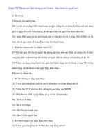
name y . Figure 7.1 sketches the contents of class Y as a so-called UML
diagram, here created with Lumpy (from Appendix H.3) with aid of the
little program class_Y_v1_UML.py. The UML diagram has two “boxes”,
one where the functions are listed, and one where the variables are
listed. Our next step is to implement this class in Python.

Fig. 7.1 UML diagram with function and data in the simple class Y for representing a

mathematical function y(t; v0 ).

Implementation. The complete code for our class Y looks as follows in
Python:
class Y:
def __init__(self, v0):
self.v0 = v0
self.g = 9.81
def value(self, t):
return self.v0*t - 0.5*self.g*t**2

A puzzlement for newcomers to Python classes is the self parameter,
which may take some efforts and time to fully understand.

345


Simpo PDF Merge and Split Unregistered Version -
33. H.P. Langtangen, A. Tveito (eds.), Advanced Topics in Computational Partial Differential Equations. Numerical
Methods and Diffpack Programming.
34. V. John, Large Eddy Simulation of Turbulent Incompressible Flows. Analytical and Numerical Results for a Class
of LES Models.
35. E. Băansch (ed.), Challenges in Scientific Computing – CISC 2002.
36. B.N. Khoromskij, G. Wittum, Numerical Solution of Elliptic Differential Equations by Reduction to the Interface.
37. A. Iske, Multiresolution Methods in Scattered Data Modelling.
38. S.-I. Niculescu, K. Gu (eds.), Advances in Time-Delay Systems.
39. S. Attinger, P. Koumoutsakos (eds.), Multiscale Modelling and Simulation.
40. R. Kornhuber, R. Hoppe, J. P´eriaux, O. Pironneau, O. Wildlund, J. Xu (eds.), Domain Decomposition Methods in
Science and Engineering.
41. T. Plewa, T. Linde, V.G. Weirs (eds.), Adaptive Mesh Refinement – Theory and Applications.

42. A. Schmidt, K.G. Siebert, Design of Adaptive Finite Element Software. The Finite Element Toolbox ALBERTA.
43. M. Griebel, M.A. Schweitzer (eds.), Meshfree Methods for Partial Differential Equations II.
44. B. Engquist, P. Lăotstedt, O. Runborg (eds.), Multiscale Methods in Science and Engineering.
45. P. Benner, V. Mehrmann, D.C. Sorensen (eds.), Dimension Reduction of Large-Scale Systems.
46. D. Kressner, Numerical Methods for General and Structured Eigenvalue Problems.
47. A. Boric¸i, A. Frommer, B. Joo, A. Kennedy, B. Pendleton (eds.), QCD and Numerical Analysis III.
48. F. Graziani (ed.), Computational Methods in Transport.
49. B. Leimkuhler, C. Chipot, R. Elber, A. Laaksonen, A. Mark, T. Schlick, C. Schutte, R. Skeel (eds.), New Algorithms for Macromolecular Simulation.
50. M. Băucker, G. Corliss, P. Hovland, U. Naumann, B. Norris (eds.), Automatic Differentiation: Applications, Theory,
and Implementations.
51. A.M. Bruaset, A. Tveito (eds.), Numerical Solution of Partial Differential Equations on Parallel Computers.
52. K.H. Hoffmann, A. Meyer (eds.), Parallel Algorithms and Cluster Computing.
53. H.-J. Bungartz, M. Schafer (eds.), Fluid-Structure Interaction.
54. J. Behrens, Adaptive Atmospheric Modeling.
55. O. Widlund, D. Keyes (eds.), Domain Decomposition Methods in Science and Engineering XVI.
56. S. Kassinos, C. Langer, G. Iaccarino, P. Moin (eds.), Complex Effects in Large Eddy Simulations.
57. M. Griebel, M.A Schweitzer (eds.), Meshfree Methods for Partial Differential Equations III.
58. A.N. Gorban, B. K´egl, D.C. Wunsch, A. Zinovyev (eds.), Principal Manifolds for Data Visualization and Dimension Reduction.
59. H. Ammari (ed.), Modeling and Computations in Electromagnetics: A Volume Dedicated to Jean-Claude N´ed´elec.
60. U. Langer, M. Discacciati, D. Keyes, O. Widlund, W Zulehner (eds.), Domain Decomposition Methods in Science
and Engineering XVII.
61. T. Mathew, Domain Decomposition Methods for the Numerical Solution of Partial Differential Equations.


Simpo PDF Merge and Split Unregistered Version -
62. F. Graziani (ed.), Computational Methods in Transport: Verification and Validation.
63. M. Bebendorf, Hierarchical Matrices. A Means to Efficiently Solve Elliptic Boundary Value Problems.
64. C.H. Bischof, H.M. Băucker, P. Hovland, U. Naumann, J. Utke (eds.), Advances in Automatic Differentiation.
65. M. Griebel, M.A. Schweitzer (eds.), Meshfree Methods for Partial Differential Equations IV.
66. B. Engquist, P. Lăotstedt, O. Runborg (eds.), Multiscale Modeling and Simulation in Science.

ă Giilcat, D.R. Emerson, K. Matsuno (eds.), Parallel Computational Fluid Dynamics 2007.
67. I.H. Tuncer, U.
68. S. Yip, T. Diaz de la Rubia (eds.), Scientific Modeling and Simulations.
69. A. Hegarty, N. Kopteva, E. O’Riordan, M. Stynes (eds.), BAIL 2008 – Boundary and Interior Layers.
70. M. Bercovier, M.J. Gander, R. Kornhuber, O. Widlund (eds.), Domain Decomposition Methods in Science and
Engineering XVIII.
71. B. Koren, C. Vuik (eds.), Advanced Computational Methods in Science and Engineering.
72. M. Peters (ed.), Computational Fluid Dynamics for Sport Simulation.
73. H.-J. Bungartz, M. Mehl, M. Schafer (eds.), Fluid Structure Interaction II – Modelling, Simulation, Optimization.
74. D. Tromeur-Dervout, G. Brenner, D.R. Emerson, J. Erhel (eds.), Parallel Computational Fluid Dynamics 2008.
75. A.N. Gorban, D. Roose (eds.), Coping with Complexity: Model Reduction and Data Analysis.
76. J.S. Hesthaven, E.M. Rønquist (eds.), Spectral and High Order Methods for Partial Differential Equations.
77. M. Holtz, Sparse Grid Quadrature in High Dimensions with Applications in Finance and Insurance.
78. Y. Huang, R. Kornhuber, O. Widlund, J. Xu (eds.), Domain Decomposition Methods in Science and Engineering
XIX.
79. M. Griebel, M.A. Schweitzer (eds.), Meshfree Methods for Partial Differential Equations V.
80. P.H. Lauritzen, C. Jablonowski, M.A. Taylor, R.D. Nair (eds.), Numerical Techniques for Global Atmospheric
Models.
81. C. Clavero, J.L. Gracia, F. Lisbona (eds.), BAIL 2010 – Boundary and Interior Layers, Computational and Asymptotic Methods.
82. B. Engquist, O. Runborg, Y.R. Tsai (eds.), Numerical Analysis and Multiscale Computations.
83. I.G. Graham, T.Y. Hou, O. Lakkis, R. Scheichl (eds.), Numerical Analysis of Multiscale Problems.
84. A. Logg, K.-A. Mardal, G.N. Wells (eds.), Automated Solution of Differential Equations by the Finite Element
Method.
85. J. Blowey, M. Jensen (eds.), Frontiers in Numerical Analysis – Durham 2010.
86. O. Kolditz, U.-J. Gorke, H. Shao, W. Wang (eds.), Thermo-Hydro-Mechanical-Chemical Processes in Fractured
Porous Media – Benchmarks and Examples.
87. S. Forth, P. Hovland, E. Phipps, J. Utke, A. Walther (eds.), Recent Advances in Algorithmic Differentiation.
88. J. Garcke, M. Griebel (eds.), Sparse Grids and Applications.
For further information on these books please have a look at our mathematics catalogue at the following URL:
www.springer.com/series/3527