RECENT ADVANCES IN ROBUST CONTROL – NOVEL APPROACHES AND DESIGN METHODSE Part 9 docx

New Practical Integral Variable Structure Controllers for Uncertain Nonlinear Systems

229
( ) , 0
T
Vx xPx P
=
> (43)
The derivative of (43) becomes

00 0 0
() [ (,) (,)] (,) (,)
TT TT T
Vx x
f
xt P P
f
xt x u
g
xtPx xP
g
xtu=+++

(44)
By means of the Lyapunov control theory(Khalil, 1996), take the control input as

0
(,)
TT
u

g
xtP
y
BP
y
=− =− (45)
and
(,) 0Qxt > and (,) 0
c
Qxt> for all
n
xR∈
and all 0t ≥ is

00
(,) (,) (,)
T
f
xtP P
f
xt Qxt+=− (46)

00
(,) (,) (,)
T
ccc
f
xtP P
f
xt Q xt+=− (47)

then

{}
00
min
() (,)
[ ( , ) ]
[ ( , ) ( , )]
( , )
( , )
TTTTTT
TTTT
TT
cc
T
c
c
V x x Q x t x x C PBB Px x PBB PCx
x Q x t C PBB P PBB PC x
xfxtPPfxtx
xQ xtx
Qxt x
λ
=− − −
=− + +
=− +
=−
≤−

(48)

Therefore the stable gain is chosen as

1
110
( ) or ( ) ( , )
T
G
y
BP HCB HC
f
xt
−
== (49)
2.3.2 Output feedback discontinuous control input
A corresponding output feedback discontinuous control input is proposed as follows:

01020
() ( )uGyyGyGSGsignS
=
−−Δ−− (50)
where
()Gy
is a nonlinear output feedback gain satisfying the relationship (37) and (49),
GΔ is a switching gain of the state,
1
G
is a feedback gain of the output feedback integral
sliding surface, and
2
G

is a switching gain, respectively as

[ ] 1, ,
i
Gg i qΔ=Δ = (51)

{
}
{}
{}
{}
11
11 110
0
11
11 110
0
max ( ) ''( . ) ( ) ( , )
( ) 0
min

min ( ) ''( . ) ( ) ( , )
( ) 0
min
i
i
i
i
i
HCB HC f xt IHCB H f xt

sign S y
II
g
HCB HC f xt IHCB H f xt
sign S y
II
−−
−−
⎧
Δ+Δ
≥>
⎪
+Δ
⎪
Δ=
⎨
Δ+Δ
⎪
≤<
⎪
+Δ
⎩
(52)

1
0G >
(53)

Recent Advances in Robust Control – Novel Approaches and Design Methods

230

{
}
2
max | ''( , )|
min{ }
dxt
G
II
=
+Δ
(55)
The real sliding dynamics by the proposed control (50) with the output feedback integral
sliding surface (35) is obtained as follows:

1
01 1 0
1
110 1 1 1 0
1
110 1 0
1
11 1
1
11
()[ ]
( )[ (,) (,) ( (,)) (,) ]
( ) [ ( , ) ( ) ]
( ) [ ( , ) ( , ) ( ) ]

( ) [
SHCBHyHy
HCB HC
f
xtx HC
f
xt HCB
g
xt u HCdxt H
y
HCB HCf xtx HCBGyy Hy
HCB HC f xt HC gxtKy y
HCB HC
−
−
−
−
−
=+
=+Δ++Δ++
=−+
+Δ+Δ
+


10 2 0 1
1
11 1
10 2 0
11

11 110
( ( , ))( ( ) ( , )]
( ) [ ''( , ) ( , ) ( ) ] ( ) ( )
[( )( ( )) ''( , )]
( ) ''( , ) ( ) ( , ) ( )
Bgxt GyGSGsignS HCdxt
HCB HC f xtCx HC gxtG y y I I Gyy
IIGSGsignS dxt
HCBHCfxty IHCBHfxty I I
−
−−
+Δ −Δ − − +
=Δ+Δ−+ΔΔ
++Δ− − +
=Δ+Δ −+Δ
10 2 0
()
( )( ( )) ''( , )
Gyy
IIGSGsignS dxt
Δ
++Δ− − +
(56)
The closed loop stability by the proposed control input with the output feedback integral
sliding surface together with the existence condition of the sliding mode will be investigated
in next Theorem 1.
Theorem 2: If the output feedback integral sliding surface (35) is designed to be stable, i.e. stable
design of ()Gy , the proposed control input (50) with Assumption A1-A10 satisfies the existence
condition of the sliding mode on the output feedback integral sliding surface and closed loop
exponential stability.

Proof; Take a Lyapunov function candidate as

00
1
()
2
T
Vy SS=
(57)
Differentiating (57) with respect to time leads to and substituting (56) into (58)

00
11
01 1 1 10 0
010200
2
10
10
()
[( ) ''( , ) ( ) ( , )] ( ) ( )
( )( ( )) ''( , )
|| || , min{|| ||}

T
T T
TT
T
Vy S S
S HCB HC f xt I HCB H f xt y S I I Gyy
SI I GS GsignS Sdxt

GS I I
GSS
εε
ε
−−
=
=Δ+Δ −+ΔΔ
++Δ−− +
≤− = +Δ
=−


0
1
2 ( )GV y
ε
=−
(58)
From (58), the second requirement to get rid of the reaching phase is satisfied. Therefore, the
reaching phase is clearly removed. There are no reaching phase problems. As a result, the
real output dynamics can be exactly predetermined by the ideal sliding output with the
matched uncertainty. Moreover from (58), the following equations are obtained as

1
() 2 () 0Vy GVy
ε
+
≤

(59)

New Practical Integral Variable Structure Controllers for Uncertain Nonlinear Systems

231

1
2
(()) ((0))
Gt
Vyt Vy e
ε
−
≤ (60)
And the second order derivative of
()Vx becomes

21
00 00 0 0 1 1 0
( ) || || ( ) ( )
TT
Vy SS SS S S HCB HCx HCx
−
=
+= + + <∞
  

 
(61)
and by Assumption A5 ( )Vx


is bounded, which completes the proof of Theorem 2.
2.3.3 Continuous approximation of output feedback discontinuous control input
Also, the control input (50) with (35) chatters from the beginning without reaching phase.
The chattering of the discontinuous control input may be harmful to the real dynamic plant
so it must be removed. Hence using the saturation function for a suitable
0
δ
, one make the
part of the discontinuous input be continuous effectively for practical application as

0
01020
00
() { ( )}
||
c
S
uGyyGSGyGsignS
S
δ
=− − − Δ +
+
(62)
The discontinuity of control input of can be dramatically improved without severe output
performance deterioration.
3. Design examples and simulation studies
3.1 Example 1: Full-state feedback practical integral variable structure controller
Consider a second order affine uncertain nonlinear system with mismatched uncertainties
and matched disturbance
2

11 1 12 1
0.1 sin ( ) 0.02sin(2.0 )xx x xx xu=− + + +



2
222 2
sin ( ) (2.0 0.5sin(2.0 )) ( , )xxx x tudxt=+ + + +

(63)

22
1212
( , ) 0.7sin( ) 0.8sin( ) 0.2( ) 2.0sin(5.0 ) 3.0dxt x x x x t=−+++ + (64)
Since (63) satisfy the Assumption A1, (63) is represented in state dependent coefficient form
as

2
1 11
1
2
2 2
2
0
0.02sin( )
10.1sin() 1
2.0 0.5sin(2.0 )
01sin()
(,)
xxx

x
u
xxt
x
dxt
⎡
⎤
−+
⎡⎤
⎡⎤ ⎡⎤⎡ ⎤
=⋅++
⎢
⎥
⎢⎥
⎢⎥ ⎢⎥⎢ ⎥
+
+
⎣⎦ ⎣⎦⎣ ⎦
⎣⎦
⎣
⎦


(65)
where the nominal parameter
0
(,)
f
xt and
0

(,)gxt and mismatched uncertainties (,)
f
xtΔ
and
(,)gxtΔ are

2
1
00
2
2
1
11 0
0.1sin ( ) 0
(,) , (,) , (,)
01 2.0
0sin()
0.02sin( )
(,)
0.2sin(2.0 )
x
fxt gxt fxt
x
x
gxt
t
−
⎡
⎤
⎡⎤ ⎡⎤

==Δ=
⎢
⎥
⎢⎥ ⎢⎥
⎣⎦ ⎣⎦
⎣
⎦
⎡⎤
Δ=
⎢⎥
⎣⎦
(66)

Recent Advances in Robust Control – Novel Approaches and Design Methods

232
To design the full-state feedback integral sliding surface, (,)
c
f
xt is selected as

00
11
(,) (,) (,)()
70 21
c
fxt fxt gxtKx
−
⎡
⎤

=− =
⎢
⎥
−−
⎣
⎦
(67)
in order to assign the two poles at 16.4772
−
and 5.5228
−
. Hence, the feedback gain
()Kx becomes

[
]
( ) 35 11Kx = (68)
The P in (14) is chosen as

100 17.5
0
17.5 5.5
P
⎡⎤
=
>
⎢⎥
⎣⎦
(69)
so as to be

2650 670
(,) (,) 0
670 196
T
cc
fxtPPfxt
−−
⎡⎤
+
=<
⎢⎥
−−
⎣⎦
(70)
Hence, the continuous static feedback gain is chosen as

[
]
0
() (,) 35 11
T
Kx g xtP== (71)
Therefore, the coefficient of the sliding surface is determined as

[
]
[
]
11112

10 1LLL== (72)
Then, to satisfy the relationship (8a) and from (8b),
0
L
is selected as

[
]
[
]
[
]
010 0 1 11121112
(,) (,)() (,) 70 21 80 11
c
LLfxtgxtKxLfxtLLLL=− − =− = + − + = (73)
The selected gains in the control input (21), (23)-(25) are as follows:

1
1
1
4.0 if 0
4.0 if 0
f
f
Sx
k
Sx
+
>

⎧
⎪
Δ=
⎨
−
<
⎪
⎩
(74a)

2
2
2
5.0 if 0
5.0 if 0
f
f
Sx
k
Sx
+
>
⎧
⎪
Δ=
⎨
−
<
⎪
⎩

(74b)

1
400.0K
=
(74c)

22
212
2.8 0.2( )Kxx=+ + (74d)
The simulation is carried out under 1[msec] sampling time and with
[]
(0) 10 5
T
x = initial
state. Fig. 1 shows four case
1
x and
2
x time trajectories (i)ideal sliding output, (ii) no
uncertainty and no disturbance (iii)matched uncertainty/disturbance, and (iv)unmatched

New Practical Integral Variable Structure Controllers for Uncertain Nonlinear Systems

233
uncertainty and matched disturbance. The three case output responses except the case (iv)
are almost identical to each other. The four phase trajectories (i)ideal sliding trajectory, (ii)no
uncertainty and no disturbance (iii)matched uncertainty/disturbance, and (iv) unmatched
uncertainty and matched disturbance are depicted in Fig. 2. As can be seen, the sliding
surface is exactly defined from a given initial condition to the origin, so there is no reaching

phase, only the sliding exists from the initial condition. The one of the two main problems of
the VSS is removed and solved. The unmatched uncertainties influence on the ideal sliding
dynamics as in the case (iv). The sliding surface ( )
f
St (i) unmatched uncertainty and
matched disturbance is shown in Fig. 3. The control input (i) unmatched uncertainty and
matched disturbance is depicted in Fig. 4. For practical application, the discontinuous input
is made be continuous by the saturation function with a new form as in (32) for a
positive 0.8
f
δ
= . The output responses of the continuous input by (32) are shown in Fig. 5
for the four cases (i)ideal sliding output, (ii)no uncertainty and no disturbance (iii)matched
uncertainty/disturbance, and (iv)unmatched uncertainty and matched disturbance. There is
no chattering in output states. The four case trajectories (i)ideal sliding time trajectory, (ii)no
uncertainty and no disturbance (iii)matched uncertainty/disturbance, and (iv) unmatched
uncertainty and matched disturbance are depicted in Fig. 6. As can be seen, the trajectories
are continuous. The four case sliding surfaces are shown in fig. 7, those are continuous. The
three case continuously implemented control inputs instead of the discontinuous input in
Fig. 4 are shown in Fig. 8 without the severe performance degrade, which means that the
continuous VSS algorithm is practically applicable. The another of the two main problems of
the VSS is improved effectively and removed.
From the simulation studies, the usefulness of the proposed SMC is proven.


Fig. 1. Four case
1
x and
2
x time trajectories (i)ideal sliding output, (ii) no uncertainty and

no disturbance (iii)matched uncertainty/disturbance, and (iv)unmatched uncertainty and
matched disturbance

Recent Advances in Robust Control – Novel Approaches and Design Methods

234



Fig. 2. Four phase trajectories (i)ideal sliding trajectory, (ii)no uncertainty and no
disturbance (iii)matched uncertainty/disturbance, and (iv) unmatched uncertainty and
matched disturbance




Fig. 3. Sliding surface ( )
f
St (i) unmatched uncertainty and matched disturbance

New Practical Integral Variable Structure Controllers for Uncertain Nonlinear Systems

235



Fig. 4. Discontinuous control input (i) unmatched uncertainty and matched disturbance

Fig. 5. Four case
1
x
and
2
x
time trajectories (i)ideal sliding output, (ii) no uncertainty and
no disturbance (iii)matched uncertainty/disturbance, and (iv)unmatched uncertainty and
matched disturbance by the continuously approximated input for a positive 0.8
f
δ
=

Recent Advances in Robust Control – Novel Approaches and Design Methods

236



Fig. 6. Four phase trajectories (i)ideal sliding trajectory, (ii)no uncertainty and no
disturbance (iii)matched uncertainty/disturbance, and (iv) unmatched uncertainty and
matched disturbance by the continuously approximated input




Fig. 7. Four sliding surfaces (i)ideal sliding surface, (ii)no uncertainty and no disturbance
(iii)matched uncertainty/disturbance, and (iv) unmatched uncertainty and matched

disturbance by the continuously approximated input

New Practical Integral Variable Structure Controllers for Uncertain Nonlinear Systems

237



Fig. 8. Three case continuous control inputs
f
c
u (i)no uncertainty and no disturbance
(ii)matched uncertainty/disturbance, and (iii) unmatched uncertainty and matched
3.2 Example 2: Output feedback practical integral variable structure controller
Consider a third order uncertain affine nonlinear system with unmatched system matrix
uncertainties and matched input matrix uncertainties and disturbance

2
11 1
2 2
22
32 33
1
33sin() 1 0 0 0
011 0 0
1 0.5sin ( ) 0 2 0.4sin ( ) 2 0.3sin(2 )
(,)
xx x
xxu
xx xxt

dxt
⎡
⎤
−−
⎡⎤
⎡⎤ ⎡⎤⎡ ⎤
⎢
⎥
⎢⎥
⎢⎥ ⎢⎥⎢ ⎥
=− ++
⎢
⎥
⎢⎥
⎢⎥ ⎢⎥⎢ ⎥
⎢
⎥
⎢⎥
⎢⎥ ⎢⎥⎢ ⎥
++ +
⎣⎦ ⎣⎦⎣ ⎦
⎣⎦
⎣
⎦



(75)

1

2
3
100
001
x
y
x
x
⎡
⎤
⎡⎤
⎢
⎥
=
⎢⎥
⎢
⎥
⎣⎦
⎢
⎥
⎣
⎦
(76)

22
11213
( , ) 0.7sin( ) 0.8sin( ) 0.2( ) 1.5sin(2 ) 1.5dxt x x x x t=−++++ (77)
where the nominal matrices
0
(,)

f
xt ,
0
(,)gxt B= and C , the unmatched system matrix
uncertainties and matched input matrix uncertainties and matched disturbance are
2
1
0
22
23
310 0 3sin()0 0
100
(,) 0 1 1, 0, C , 0 0 0
001
102 2 0.5sin()00.4sin()
x
fxt B f
xx
−−
⎡
⎤
⎡⎤⎡⎤
⎡⎤
⎢
⎥
⎢⎥⎢⎥
=− = = Δ=
⎢⎥
⎢
⎥

⎢⎥⎢⎥
⎣⎦
⎢
⎥
⎢⎥⎢⎥
⎣⎦⎣⎦
⎣
⎦


Recent Advances in Robust Control – Novel Approaches and Design Methods

238

1
00
(,) 0 , (,) 0
0.3sin(2 )
(,)
gxt dxt
t
dxt
⎡
⎤
⎡⎤
⎢
⎥
⎢⎥
Δ= =
⎢

⎥
⎢⎥
⎢
⎥
⎢⎥
⎣⎦
⎣
⎦
. (78)
The eigenvalues of the open loop system matrix
0
(,)
f
xt are -2.6920, -2.3569, and 2.0489,
hence
0
(,)
f
xt is unstable. The unmatched system matrix uncertainties and matched input
matrix uncertainties and matched disturbance satisfy the assumption A3 and A8 as

2
1
1
22
23
3sin ( ) 0
1
" 0 0 , 0.15sin(2 ) 0.15 1, "( , ) ( , )
2

0.5sin ( ) 0.4sin ( )
x
f
It dxtdxt
xx
⎡⎤
−
⎢⎥
Δ= Δ= ≤ < =
⎢⎥
⎢⎥
⎣⎦
(79)
disturbance by the continuously approximated input for a positive 0.8
f
δ
=

To design the output feedback integral sliding surface,
(,)
c
f
xt is designed as

00
31 0
(,) (,) () 0 1 1
19 0 30
c
fxt fxt BGyC

−
⎡
⎤
⎢
⎥
=− =−
⎢
⎥
⎢
⎥
−−
⎣
⎦
(80)

in order to assign the three stable pole to (,)
c
fxt at 30.0251
−
and 2.4875 0.6636i
−
± . The
constant feedback gain is designed as

[
]
{
}
1
() 2 [1 0 2] 19 0 30GyC

−
=−−
(81)

[
]
() 10 16Gy∴=
(82)
Then, one find
[
]
11112
Hhh= and
[
]
00102
Hhh= which satisfy the relationship (37) as

11 01 12 02 12
0, 19 , 30hhhhh
=
== (83)

One select
12
1h = ,
01
19h
=
, and

02
30h
=
. Hence
112
22HCB h
=
= is a non zero satisfying
A4. The resultant output feedback integral sliding surface becomes

[] [ ]
101
0
202
1
0 1 19 30
2
yy
S
yy
⎧
⎫
⎡
⎤⎡⎤
⎪
⎪
=+
⎨
⎬
⎢

⎥⎢⎥
⎪
⎪
⎣
⎦⎣⎦
⎩⎭
(84)
where

01 1
0
()
t
yy
d
τ
τ
=
∫
(85)

02 2 2
0
() (0)/30
t
yydy
ττ
=−
∫
(86)

The output feedback control gains in (50), (51)-(55) are selected as follows:

New Practical Integral Variable Structure Controllers for Uncertain Nonlinear Systems

239

01
1
01
1.6 if 0
1.6 if 0
Sy
g
Sy
+
>
⎧
Δ=
⎨
−
<
⎩
(87a)

02
2
02
1.7 if 0
1.7 if 0

Sy
g
Sy
+
>
⎧
Δ=
⎨
−
<
⎩
(87b)

1
500.0G = (87c)

22
212
3.2 0.2( )G
yy
=+ + (87d)
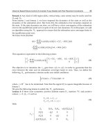
The simulation is carried out under 1[msec] sampling time and with
[]
(0) 10 0.0 5
T
x =
initial state. Fig. 9 shows the four case two output responses of
1
y
and

2
y
(i)ideal sliding
output, (ii) with no uncertainty and no disturbance, (iii)with matched uncertainty and
matched disturbance, and (iv) with ummatched uncertainty and matched disturbance. The
each two output is insensitive to the matched uncertainty and matched disturbance, hence is
almost equal, so that the output can be predicted. The four case phase trajectories (i)ideal
sliding trajectory, (ii) with no uncertainty and no disturbance, (iii)with matched uncertainty
and matched disturbance, and (iv) with ummatched uncertainty and matched disturbance
are shown in Fig. 10. There is no reaching phase and each phase trajectory except the case
(iv) with ummatched uncertainty and matched disturbance is almost identical also. The
sliding surface is exactly defined from a given initial condition to the origin. The output
feedback integral sliding surfaces (i) with ummatched uncertainty and matched disturbance
is depicted in Fig. 11. Fig. 12 shows the control inputs (i)with unmatched uncertainty and
matched disturbance. For practical implementation, the discontinuous input can be made
continuous by the saturation function with a new form as in (32) for a positive
0
0.02
δ
=
. The
output responses by the continuous input of (62) are shown in Fig. 13 for the four cases
(i)ideal sliding output, (ii)no uncertainty and no disturbance (iii)matched
uncertainty/disturbance, and (iv)unmatched uncertainty and matched disturbance. There is
no chattering in output responses. The four case trajectories (i)ideal sliding time trajectory,
(ii)no uncertainty and no disturbance (iii)matched uncertainty/disturbance, and (iv)
unmatched uncertainty and matched disturbance are depicted in Fig. 14. As can be seen, the
trajectories are continuous. The four case sliding surfaces are shown in fig. 15, those are
continuous also. The three case continuously implemented control inputs instead of the
discontinuous input in Fig. 12 are shown in Fig. 16 without the severe performance loss,

which means that the chattering of the control input is removed and the continuous VSS
algorithm is practically applicable to the real dynamic plants. From the above simulation
studies, the proposed algorithm has superior performance in view of the no reaching phase,
complete robustness, predetermined output dynamics, the prediction of the output, and
practical application. The effectiveness of the proposed output feedback integral nonlinear
SMC is proven.
Through design examples and simulation studies, the usefulness of the proposed practical
integral nonlinear variable structure controllers is verified. The continuous approximation
VSS controllers without the reaching phase in this chapter can be practically applicable to
the real dynamic plants.

Recent Advances in Robust Control – Novel Approaches and Design Methods

240



Fig. 9. Four case two output responses of
1
y
and
2
y
(i)ideal sliding output, (ii) with no
uncertainty and no disturbance, (iii)with matched uncertainty and matched disturbance,
and (iv) with ummatched uncertainty and matched disturbance



Fig. 10. Four phase trajectories (i)ideal sliding trajectory, (ii)no uncertainty and no

disturbance (iii)matched uncertainty/disturbance, and (iv)unmatched uncertainty and
matched disturbance

New Practical Integral Variable Structure Controllers for Uncertain Nonlinear Systems

241






Fig. 11. Sliding surface
0
()St (i) unmatched uncertainty and matched disturbance




Fig. 12. Discontinuous control input (i) unmatched uncertainty and matched disturbance

Recent Advances in Robust Control – Novel Approaches and Design Methods

242





Fig. 13. Four case

1
y
and
2
y
time trajectories (i)ideal sliding output, (ii) no uncertainty and
no disturbance (iii)matched uncertainty/disturbance, and (iv)unmatched uncertainty and
matched disturbance by the continuously approximated input for a positive
0
0.02
δ
=



Fig. 14. Four phase trajectories (i)ideal sliding trajectory, (ii)no uncertainty and no
disturbance (iii)matched uncertainty/disturbance, and (iv) unmatched uncertainty and
matched disturbance by the continuously approximated input

New Practical Integral Variable Structure Controllers for Uncertain Nonlinear Systems

243





Fig. 15. Four sliding surfaces (i)ideal sliding surface , (ii)no uncertainty and no disturbance
(iii)matched uncertainty/disturbance, and (iv) unmatched uncertainty and matched
disturbance by the continuously approximated input

Fig. 16. Three case continuous control inputs
0c
u
(i)no uncertainty and no disturbance
(ii)matched uncertainty/disturbance, and (iii) unmatched uncertainty and matched
disturbance by the continuously approximated input for a positive
0
0.02
δ
=


Recent Advances in Robust Control – Novel Approaches and Design Methods

244
4. Conclusion
In this chapter, a new practical robust full-state(output) feedback nonlinear integral variable
structure controllers with the full-state(output) feedback integral sliding surfaces are
presented based on state dependent nonlinear form for the control of uncertain more affine
nonlinear systems with mismatched uncertainties and matched disturbance. After an affine
uncertain nonlinear system is represented in the form of state dependent nonlinear system, a
systematic design of the new robust integral nonlinear variable structure controllers with
the full-state(output) feedback (transformed) integral sliding surfaces are suggested for
removing the reaching phase. The corresponding (transformed) control inputs are proposed.
The closed loop stabilities by the proposed control inputs with full-state(output) feedback
integral sliding surface together with the existence condition of the sliding mode on the
selected sliding surface are investigated in Theorem 1 and Theorem 2 for all mismatched
uncertainties and matched disturbance. For practical application of the continuous

discontinuous VSS, the continuous approximation being different from that of (Chern &
Wu, 1992) is suggested without severe performance degrade. The two practical algorithms,
i.e., practical full-state feedback integral nonlinear variable structure controller with the full-
state feedback transformed input and the full-state feedback sliding surface and practical
output feedback integral nonlinear variable structure controller with the output feedback
input and the output feedback transformed sliding surface are proposed. The outputs by the
proposed inputs with the suggested sliding surfaces are insensitive to only the matched
uncertainty and disturbance. The unmatched uncertainties can influence on the ideal sliding
dynamics, but the exponential stability is satisfied. The two main problems of the VSS, i.e.,
the reaching phase at the beginning and the chattering of the input are removed and solved.
5. References
Adamy, J. & Flemming, A. (2004). Soft Variable Structure Control: a Survey. Automatica,
vol.40, pp.1821-1844.
Anderson, B. D. O. & More, J. B. (1990) Optimal Control, Prentice-Hall.
Bartolini, G. & Ferrara, A. (1995). On Multi-Input Sliding Mode Control of Uncertain
Nonlinear Systems. Proceeding of IEEE 34th CDC, p.2121-2124.
Bartolini, G., Pisano, A. & Usai, E. (2001). Digital Second-Order Sliding Mode Control for
Uncertain Nonlinear Systems. Automatica, vol.37 pp.1371-1377.
Cai, X., Lin, R., and Su, SU., (2008). Robust stabilization for a class of Nonlinear Systems.
Proceeding of IEEE CDC pp.4840-4844, 2008.
Chen, W. H., Ballance, D. J. & Gawthrop, P. J. (2003). Optimal Control of Nonlinear
System:A Predictive Control Approach. Automatica, vol. 39, pp633-641.
Chern, T. L. & Wu, Y. C., (1992). An Optimal Variable Structure Control with Integral
Compensation for Electrohydraulic Position Servo Control Systems. IEEE T.
Industrial Electronics, vol.39, no.5 pp460-463.
Decarlo, R. A., Zak, S. H., & Mattews, G. P., (1988). Variable Structure Control of Nonlinear
Multivariable Systems: A Tutorial. Proceeding of IEEE, Vol. 76, pp.212-232.
Drazenovic, B., (1969). The invariance conditions in variable structure systems, Automatica,
Vol. 5, pp.287-295.

New Practical Integral Variable Structure Controllers for Uncertain Nonlinear Systems

245
Gutman, S. (1979). Uncertain dynamical Systems:A Lyapunov Min-Max Approach. IEEE
Trans. Autom. Contr, Vol. AC-24, no. 1, pp.437-443.
Horowitz, I. (1991). Survey of Quantitative Feedback Theory(QFT). Int. J. Control, vol.53,
no.2 pp.255-291.
Hu, X. & Martin, C. (1999). Linear Reachability Versus Global Stabilization. IEEE Trans.
Autom. Contr, AC-44, no. 6, pp.1303-1305.
Hunt, L. R., Su, R. & Meyer, G. (1987). Global Transformations of Nonlinear Systems," IEEE
Trans. Autom. Contr, Vol. AC-28, no. 1, pp.24-31.
Isidori, A., (1989). Nonlinear Control System(2e). Springer-Verlag.
Khalil, H. K. (1996). Nonlinear Systems(2e). Prentice-Hall.
Kokotovic, P. & Arcak, M. (2001). Constructive Nonlinear Control: a Historical Perspective.
Automatica, vol.37, pp.637-662.
Lee, J. H. & Youn, M. J., (1994). An Integral-Augmented Optimal Variable Structure control
for Uncertain dynamical SISO System, KIEE(The Korean Institute of Electrical
Engineers), vol.43, no.8, pp.1333-1351.
Lee, J. H. (1995). Design of Integral-Augmented Optimal Variable Structure Controllers, Ph.
D. dissertation, KAIST.
Lee, J. H., (2004). A New Improved Integral Variable Structure Controller for Uncertain
Linear Systems. KIEE, vol.43, no.8, pp.1333-1351.
Lee, J. H., (2010a). A New Robust Variable Structure Controller for Uncertain Affine
Nonlinear Systems with Mismatched Uncertainties," KIEE, vol.59, no.5, pp.945-949.
Lee, J. H., (2010b). A Poof of Utkin's Theorem for a MI Uncertain Linear Case," KIEE, vol.59,
no.9, pp.1680-1685.
Lee, J. H., (2010c). A MIMO VSS with an Integral-Augmented Sliding Surface for Uncertain
Multivariable Systems
," KIEE, vol.59, no.5, pp.950-960.
Lijun, L. & Chengkand, X., (2008). Robust Backstepping Design of a Nonlinear Output

Feedback System, Proceeding of IEEE CDC 2008, pp.5095-5099.
Lu, X. Y. & Spurgeon, S. K. (1997). Robust Sliding Mode Control of Uncertain Nonlinear
System. System & control Letters, vol.32, pp.75-90.
Narendra, K. S. (1994). Parameter Adaptive Control-the End or the Beginning? Proceeding of
33rd IEEE CDC.
Pan, Y. D. Kumar, K. D. Liu, G. J., & Furuta, K. (2009). Design of Variable Structure Control
system with Nonlinear Time Varying Sliding Sector. IEEE Trans. Autom. Contr, AC-
54, no. 8, pp.1981-1986.
Rugh, W. J. & Shamma, J., (2000). Research on Gain Scheduling. Automatica, vol.36, pp.1401-
1425.
Slottine, J. J. E. & Li, W., (1991). Applied Nonlinear Control, Prentice-Hall.
Sun, Y. M. (2009). Linear Controllability Versus Global Controllability," IEEE Trans. Autom.
Contr, AC-54, no. 7, pp.1693-1697.
Tang, G. Y., Dong, R., & Gao, H. W. (2008). Optimal sliding Mode Control for Nonlinear
System with Time Delay. Nonlinear Analysis: Hybrid Systems, vol.2, pp891-899.
Toledo, B. C., & Linares, R. C., (1995). On Robust Regulation via Sliding Mode for Nonlinear
Systems, System & Control Letters, vol.24, pp.361-371.
Utkin, V. I. (1978). Sliding Modes and Their Application in Variable Structure Systems. Moscow,
1978.

Recent Advances in Robust Control – Novel Approaches and Design Methods

246
Vidyasagar, M. (1986). New Directions of Research in Nonlinear System Theory. Proc. of the
IEEE, Vol.74, No.8, (1986), pp.1060-1091.
Wang, Y., Jiang, C., Zhou, D., & Gao, F. (2007). Variable Structure Control for a Class of
Nonlinear Systems with Mismatched Uncertainties. Applied Mathematics and
Computation, pp.1-14.
Young, K.D., Utkin, V.I., & Ozguner, U, (1996). A Control Engineer's Guide to Sliding Mode
Control. Proceeding of 1996 IEEE Workshop on Variable Structure Systems, pp.1-14.

Zheng, Q. & Wu, F. Lyapunov Redesign of Adpative Controllers for Polynomial Nonlinear
systems," (2009). Proceeding of IEEE ACC 2009, pp.5144-5149.
11
New Robust Tracking and Stabilization Methods
for Significant Classes of Uncertain
Linear and Nonlinear Systems
Laura Celentano
Dipartimento di Informatica e Sistemistica
Università degli Studi di Napoli Federico II, Napoli,
Italy
1. Introduction
There exist many mechanical, electrical, electro-mechanical, thermic, chemical, biological
and medical linear and nonlinear systems, subject to parametric uncertainties and non
standard disturbances, which need to be efficiently controlled. Indeed, e.g. consider the
numerous manufacturing systems (in particular the robotic and transport systems,…) and
the more pressing requirements and control specifications in an ever more dynamic society.
Despite numerous scientific papers available in literature (Porter and Power, 1970)-(Sastry,
1999), some of which also very recent (Paarmann, 2001)-(Siciliano and Khatib, 2009), the
following practical limitations remain:
1. the considered classes of systems are often with little relevant interest to engineers;
2. the considered signals (references, disturbances,…) are almost always standard
(polynomial and/or sinusoidal ones);
3. the controllers are not very robust and they do not allow satisfying more than a single
specification;
4. the control signals are often excessive and/or unfeasible because of the chattering.
Taking into account that a very important problem is to force a process or a plant to track
generic references, provided that sufficiently regular, e.g. the generally continuous
piecewise linear signals, easily produced by using digital technologies, new theoretical
results are needful for the scientific and engineering community in order to design control
systems with non standard references and/or disturbances and/or with ever harder

specifications.
In the first part of this chapter, new results are stated and presented; they allow to design a
controller of a SISO process, without zeros, with measurable state and with parametric
uncertainties, such that the controlled system is of type one and has, for all the possible
uncertain parameters, assigned minimum constant gain and maximum time constant or
such that the controlled system tracks with a prefixed maximum error a generic reference
with limited derivative, also when there is a generic disturbance with limited derivative, has
an assigned maximum time constant and guarantees a good quality of the transient.
The proposed design techniques use a feedback control scheme with an integral action (Seraj
and Tarokh, 1977), (Freeman and Kokotovic, 1995) and they are based on the choice of a

Recent Advances in Robust Control – Novel Approaches and Design Methods

248
suitable set of reference poles, on a proportionality parameter of these poles and on the
theory of externally positive systems (Bru and Romero-Vivò, 2009).
The utility and efficiency of the proposed methods are illustrated with an attractive and
significant example of position control.
In the second part of the chapter it is considered the uncertain pseudo-quadratic systems of
the type
12
1
(,,) (,,) (,,,)
m
ii
i
yFyypu Fyypyyftyyp
=
⎡⎤
=+ +

⎢⎥
⎣⎦
∑
     
, where tR
∈
is the time,
m
yR∈ is
the output,
r
uR∈ is the control input,
p
R
μ
∈℘⊂ is the vector of uncertain parameters,
with
℘
compact set,
1
mr
FR
×
∈ is limited and of rank m ,
2
mxm
i
FR∈ is limited and
m
f

R∈ is
limited and models possible disturbances and/or particular nonlinearities of the system.
For this class of systems, including articulated mechanical systems, several theorems are
stated which easily allow to determine robust control laws of the PD type, with a possible
partial compensation, in order to force
y
and
y

to go to rectangular neighbourhoods (of
the origin) with prefixed areas and with prefixed time constants characterizing the
convergence of the error. Clearly these results allow also designing control laws to take and
hold a generic articulated system in a generic posture less than prefixed errors also in the
presence of parametric uncertainties and limited disturbances.
Moreover the stated theorems can be used to determine simple and robust control laws in
order to force the considered class of systems to track a generic preassigned limited in
“acceleration” trajectory, with preassigned majorant values of the maximum “position
and/or velocity” errors and preassigned increases of the time constants characterizing the
convergence of the error.
Part I
2. Problem formulation and preliminary results
Consider the SISO n-order system, linear, time-invariant and with uncertain parameters,
described by
,xAxBu yCxd
=
+=+

, (1)
where:
n

xR∈ is the state, uR
∈
is the control signal, dR
∈
is the disturbance or, more in
general, the effect
d
y
of the disturbance d on the output,
y
R∈ is the
output,
,AAA
−+
≤≤ BBB
−
+
≤
≤ and CCC
−
+
≤≤ .
Suppose that this process is without zeros, is completely controllable and that the state is
measurable.
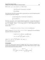
Moreover, suppose that the disturbance
d and the reference r are continuous signals with
limited first derivative (see Fig. 1).
A main goal is to design a linear and time invariant controller such that:
1. ,, ,, ,AAA BBB CCC
−+ −+ −+

∀∈ ∀∈ ∀∈
⎡⎤⎡⎤ ⎡⎤
⎣⎦⎣⎦ ⎣⎦
the control system is of type one, with
constant gain
ˆ
vv
KK≥ and maximum time constant
max max
ˆ
τ
τ
≤
, where
ˆ
v
K and
max
ˆ
τ
are
design specifications, or
2.
condition 1. is satisfied and, in addition, in the hypothesis that the initial state of the
control system is null and that
(0) (0) 0rd
−
=
, the tracking error
()et

satisfies relation
New Robust Tracking and Stabilization Methods
for Significant Classes of Uncertain Linear and Nonlinear Systems

249

[]
0,
1
ˆˆ
() , 0, (), (): max ( ) ( )
ˆ
rd rd rd
t
v
et t rt dt r d
K
σ
δ
δσσδ
−
−−
∈
≤∀≥∀ = −≤




, (2)

0 1 2 3 4 5 6 7 8 9 10
-2
-1
0
1
2
t
u, d
0 1 2 3 4 5 6 7 8 9 10
-2
0
2
t
u, d
.
.
.
.
0 1 2 3 4 5 6 7 8 9 10
-2
0
2
t
u, d
0 1 2 3 4 5 6 7 8 9 10
-2
0
2
t
u, d

.
.
.
.

Fig. 1. Possible reference or disturbance signals with limited derivative.
where the maximum variation velocity
ˆ
rd
δ
−


of
() ()rt dt−
is a design specification.
Remark 1. Clearly if the initial state of the control system is not null and/or
(0) (0) 0rd−≠

(and/or, more in general,
() ()rt dt−
has discontinuities), the error
()et
in (2) must be
considered unless of a “free evolution“, whose practical duration can be made minus that a
preassigned settling time
ˆ
a
t .
Remark 2. If disturbance d does not directly act on the output

y
, said
d
y
its effect on the
output, in (2)
d

must be substituted with
d
y

.
This is one of the main and most realistic problem not suitable solved in the literature of
control (Porter et al., 1970)-(Sastry, 1999).
There exist several controllers able to satisfy the 1. and/or 2 specifications. In the following,
for brevity, is considered the well-known state feedback control law with an integral (I)
control action (Seraj and Tarokh, 1977), (Freeman and Kokotovic, 1995).
By posing

1
111
1
1
( ) ( ) , , , ,

nnn
nn
n
b

Gs CsI A B a a a a a a b b b
sas a
−
−+−+−+
−
=− = ≤≤ ≤≤ ≤≤
+++
, (3)
in the Laplace domain the considered control scheme is the one of Fig. 2.

1
+
n
k
s
1
1

nn
n
b
s
as a
−
+
++
12
12

nn

n
ks k s k
−−
+
++
r

Fig. 2. State feedback control scheme with an I control action.
Remark 3. It is useful to note that often the state-space model of the process (1) is already in
the corresponding companion form of the input-output model of the system (3) (think to the
case in which this model is obtained experimentally by using e.g. Matlab command
invfreqs); on the contrary, it is easy to transform the interval uncertainties of
,,ABC into
the ones (even if more conservative) of
,
i
ab.

Recent Advances in Robust Control – Novel Approaches and Design Methods

250
Moreover note that almost always the controller is supplied with an actuator having gain
a
g . In this case it can be posed
a
bbg
←
and also consider the possible uncertainty of
a
g .

Finally, it is clear that, for the controllability of the process, the parameter b must be always
not null. In the following, without loss of generality, it is supposed that
0. b
−
>
Remark 4. In the following it will be proved that, by using the control scheme of Fig. 2, if (2)
is satisfied then the overshoot of the controlled system is always null.
From the control scheme of Fig. 2 it can be easily derived that

1
11
1
11 1
() ()
() (()())()(()())
() ()
nn
nn
nn
nn n
sabks abk
Ess RsDs SsRsDs
s a bk s a bk s bk
−
+
+
++ +++
=−=−
++ +++ +
. (4)

If it is posed that

1 1
11 1 1 1
() ( ) ( )
nn nn
nn n nn
d s s a bk s a bk s bk s d s d s d
+ +
+
+
=++ +++ + =+ +++, (5)
from (4) and by noting that the open loop transfer function is

1 1
11
11 1
()
() ()( )
n n
nn nn
nn n
kb d
Fs
ss a bks a bk ss ds d
+ +
−−
==
+ + ++ + + ++
, (6)

the sensitivity function
()Ss of the error and the constant gain
v
K turn out to be:

1
111
1
11

() , .

nn
nnn
v
nn
nn n n n
sds d d bk
Ss s K
sds dsd dabk
−
++
+
+
+++
===
++++ +
(7)
Moreover the sensitivity function
()Ws of the output is

1
1
11
()

n
nn
nn
d
Ws
sds dsd
+
+
+
=
++++
. (8)
Definition 1. A symmetric set of 1n
+
negative real part complex numbers
{
}
12 1
, , ,
n
Ppp p
+
= normalized such that
1

1
()1
n
i
i
p
+
=
∏
−= is said to be set of reference poles.
Let be

1
11
()
nn
nn
ds s ds ds d
+
+
=+ +++ (9)
the polynomial whose roots are a preassigned set of reference poles
P . By choosing the
poles
P of the control system equal to P
ρ
, with
ρ
positive , it is

11
11
()
nnnn
nn
ds s ds ds d
ρρρ
++
+
=+ ++ + . (10)
Moreover, said ( )
p
st the impulsive response of the system having transfer function

1
1
1
11
1
() ()

nn
n
p
nn
nn
sds d
Ss Ss
ssdsdsd
−

+
+
+++
==
++++
, (11)
from (4) and from the first of (7) it is
New Robust Tracking and Stabilization Methods
for Significant Classes of Uncertain Linear and Nonlinear Systems

251

()
1
0
() ()()(), () ()
t
ppp
e t s r t d t d where s t S s
ττ ττ
−
≤−−− =
∫


L
, (12)
from which, if all the poles of ( )
p
Ss have negative real part, it is

1
()
rd
v
et
H
δ
−
≤


, (13)
where

[]
0,
0
1
,max()()
()
v
rd
t
p
Hrd
sd
σ
δ
σσ

ττ
∞
−
∈
==−
∫




. (14)
Remark 5. Note that, while the constant gain
v
K allows to compute the steady-state
tracking error to a ramp reference signal,
v
H , denoted absolute constant gain, allows to obtain
t∀ an excess estimate of the tracking error to a generic reference with derivative. On this
basis, it is very interesting from a theoretical and practical point of view, to establish the
conditions for which
vv
HK= .
In order to establish the condition necessary for the equality of the absolute constant gain
v
H with the constant gain
v
K and to provide some methods to choose the poles
P
and
ρ

,
the following preliminary results are necessary. They concern the main parameters of the
sensitivity function
()Ws of the output and the externally positive systems, i.e. the systems
with non negative impulse response.
Theorem 1. Let be s ,
s
t ,
a
t ,
s
ω
the overshoot, the rise time, the settling time and the upper
cutoff angular frequency of

11
1
11
()
()
nn
nn
nn
dd
Ws
ds s ds ds d
++
+
+
==

++++
(15)
and

1
1
1 1
1
11
0
1
,, ()

()
nn
n n
vv p
nn
n nn
p
dsdsd
K H where s t
dsdsdsd
sd
ττ
−
−
+
∞
+

+
⎛⎞
+++
== =
⎜⎟
++++
⎝⎠
∫
L
, (16)
then the corresponding values of
,,, , ,
sa s v v
st t K H
ω
when 1
ρ
≠
turn out to be:

,,, , ,
sa
sa ssvvvv
tt
ss t t K K H H
ω
ρω ρ ρ
ρρ
== = = = =
. (17)

Proof. By using the change of scale property of the Laplace transform, (8) and (10) it is

1
1
1
1
11
11
1
1
1
1
11
1
() () ()
1
= ( ).

n
n
nnnn
nn
n
nn
nn
td
w
s
sds dsd
d

wt
s
sds dsd
ρ
ρ
ρρ
ρρρ ρρρ
+
−
+
−
++
+
−
+
−
+
+
⎛⎞
⎛⎞
=
=
⎜⎟
⎜⎟
++++
⎝⎠
⎝⎠
⎛⎞
=
⎜⎟

++++
⎝⎠
L
L
(18)

Recent Advances in Robust Control – Novel Approaches and Design Methods

252
By using again the change of scale property of the Laplace transform, by taking into
account (10) and (11) it is

1
1
1
11
11
1
1
1
1
11
() ()
() () ()

= ( ),

nnn
n
p

nnnn
nn
nn
n
p
nn
nn
tsdsd
s
sds dsd
sds d
st
sds dsd
ρρρ ρ
ρ
ρ
ρρρ ρρρ
−
−
++
+
−
−
+
+
⎛⎞
⎛⎞
+++
=
=

⎜⎟
⎜⎟
++++
⎝⎠
⎝⎠
⎛⎞
+++
=
⎜⎟
++++
⎝⎠
L
L
(19)
from which

()
00 0
11
()
pp p
t
sd s dt stdt
ττ
ρρ ρ
∞∞ ∞
⎛⎞
==
⎜⎟
⎝⎠

∫∫ ∫
. (20)
From the second of (7) and from (10), (14), (18), (20) the proof easily follows.
Theorem 2. Let be ,,1,2, ,,
iii
aaai n
−+
∈=
⎡⎤
⎣⎦
and ,bbb
−+
∈
⎡
⎤
⎣
⎦
the nominal values of the
parameters of the process and
ˆ
ˆ
PP
ρ
= the desired nominal poles. Then the parameters of
the controller, designed by using the nominal parameters of the process and the nominal
poles, turn out to be:

1
1
1

ˆˆ
ˆˆ
,1,2, ,,
in
ii n
in
da d
kink
bb
ρρ
+
+
+
−
== =. (21)
Moreover the polynomial of the effective poles and the constant gain are:

ˆ
ˆ
() () () ()ds ds hns s
δ
=+ + (22)

1
11
ˆ
ˆ
ˆ
ˆ
11

n
nn
v
n
nn
nn nn
dd
K
aa
ad ad
hh
ρ
ρ
+
++
==
−
+−+
++
, (23)
where:

111
1111
ˆˆˆˆ
ˆˆˆ
( )
nn nnnn
nn nn
dssds dsd sds dsd

ρρρ
+++
+
+
=+ ++ + =+ +++ (24)

1
1111
ˆˆˆ
ˆˆ ˆ ˆ
()
nnnn
nn nn
ns d s d s d ds ds d
ρρρ
+
+
+
=+++ =+++
(25)

1
1
1
111
,()
, , , .
n
n
n

n
nnn
babab
hsa sa s
aa
bbb
bbb a a a a a a
δ
⎛⎞
⎛⎞
ΔΔΔΔΔ
==−++−
⎜⎟
⎜⎟
⎝⎠
⎝⎠
Δ= − Δ = − Δ = −
(26)
Proof. The proof is obtained by making standard manipulations starting from (5), from the
second of (7) and from (10). For brevity it has been omitted.
Theorem 3. The coefficients d of the polynomial

11
max
ˆˆ
ˆ
() [ 1], 1
nnn
ds s s s s d
α

ατ
+−
−= + = , (27)
New Robust Tracking and Stabilization Methods
for Significant Classes of Uncertain Linear and Nonlinear Systems

253
where ()ds is the polynomial (5) or (22), are given by using the affine transformation

1
1
2
2
2
12
1
1
1
.
1
ˆ
ˆ
10.0
1
ˆˆ
1
1.0
ˆ
2

1
ˆˆ ˆ
1
.1
ˆ
12
11
ˆˆˆˆ
.
11
nn
n
n
nn
n
n
n
an
a
d
nn
an
nn
bn
nn
nn
χ
α
αχ

α
αα χ
α
αααχ
−−
−
+
+
+
=+
−
+
−−
−
−
⎛⎞
⎡⎤
⎜⎟
⎝⎠
⎢⎥
⎛⎞
⎢⎥
⎜⎟
⎡⎤ ⎛ ⎞
⎢⎥
⎝⎠
⎜⎟
⎢⎥
⎝⎠
⎢⎥

⎢⎥
⎢⎥
⎢⎥
⎢⎥
⎛⎞ ⎛⎞
⎢⎥
⎢⎥
⎛⎞
⎜⎟ ⎜⎟
⎢⎥
⎝⎠ ⎝⎠
⎢⎥
⎜⎟
⎢⎥
⎣⎦ ⎝ ⎠
⎢⎥
⎛⎞ ⎛ ⎞ ⎛⎞
⎢⎥
⎜⎟ ⎜ ⎟ ⎜⎟
⎢⎥
⎣⎝⎠ ⎝ ⎠ ⎝⎠ ⎦
1
,
1
ˆ
1
n
n
n
n

α
+
+
+
⎡
⎤
⎢
⎥
⎢
⎥
⎢
⎥
⎢
⎥
⎢
⎥
⎢
⎥
⎢
⎥
⎢
⎥
⎢
⎥
⎢
⎥
⎢
⎥
⎛⎞
⎢

⎥
⎜⎟
⎣
⎝⎠⎦
(28)
where

1
1
2
2
12
1
1
1
1
.
10.00
ˆ
1.00
ˆ
ˆ
ˆ
ˆ

.1
.
ˆˆ
.10
ˆ

ˆ
12
11
ˆˆˆ
.1
11
nn
n
n
nn
n
k
k
nn
nn
k
nn
nn
α
χ
χ
αα
χ
ααα
−−
+
+
−
=
−

−−
−
−
⎡⎤
⎢⎥
⎛⎞
⎢⎥
⎜⎟
⎢⎥
⎝⎠
⎡
⎤
⎡⎤
⎢⎥
⎢
⎥
⎢⎥
⎢⎥
⎢
⎥
⎢⎥
⎢⎥
⎢
⎥
⎢⎥
⎛⎞ ⎛⎞
⎢⎥
⎢
⎥
⎢⎥

⎜⎟ ⎜⎟
⎣⎦ ⎝ ⎠ ⎝ ⎠
⎣
⎦
⎢⎥
⎢⎥
⎛⎞ ⎛ ⎞ ⎛⎞
⎢⎥
⎜⎟ ⎜ ⎟ ⎜⎟
⎢⎥
⎣⎝⎠ ⎝ ⎠ ⎝⎠ ⎦
(29)
Proof. The proof is obtained by making standard manipulations and for brevity it has been
omitted.
Now, as pre-announced, some preliminary results about the externally positive systems are
stated.
Theorem 4. Connecting in series two or more SISO systems, linear, time-invariant and
externally positive it is obtained another externally positive system.
Proof. If
1
()Ws and
2
()Ws are the transfer functions of two SISO externally positive systems
then
(
)
1
11
() () 0wt Ws
−

=≥L
and
(
)
1
22
() () 0wt Ws
−
=
≥L
. From this and considering that

()
1
12 1 2
0
() () () ( ) ()
t
wt W sW s w t w d
τ
ττ
−
==−
∫
L (30)
the proof follows.
Theorem 5. A third-order SISO linear and time-invariant system with transfer function

()
22

1
()
()
Ws
sp s
α
ω
=
−−+
⎡
⎤
⎣
⎦
, (31)
i.e. without zeros, with a real pole
p
and a couple of complex poles j
α
ω
±
, is externally
positive iff
p
α
≤ , i.e. iff the real pole is not on the left of the couple of complex poles.
Proof. By using the translation property of the Laplace transform it is