Lecture Introduction to Machine learning and Data mining: Lesson 10
Bạn đang xem bản rút gọn của tài liệu. Xem và tải ngay bản đầy đủ của tài liệu tại đây (1.86 MB, 25 trang )
Introduction to
Machine Learning and Data Mining
(Học máy và Khai phá dữ liệu)
Khoat Than
School of Information and Communication Technology
Hanoi University of Science and Technology
2022
Contents
¡ Introduction to Machine Learning & Data Mining
¡ Supervised learning
¡ Unsupervised learning
¡ Probabilistic modeling
¡ Regularization
¡ Practical advice
2
Revisiting overfiting
3
¡The complexity of the learned function: 𝑦 = 𝑓# ,
ă
! the more
For a given training data D: the more complicated 𝑓,
possibility
that 𝑓! fits D better.
Overfitting
For a given D: there exist many functions that fit D perfectly (i.e.,
ng set size,
complexity
(e.g., degree of polynomials)
no vary
errorHon
D).
ă
Bishop,
Figure 1.5 those functions might generalize badly.
ă However,
f(x)
1
ERMS
Error
Training
Test
0.5
0
0
3
M
6
Complexity
9
x
The Bias-Variance Decomposition
4
¡ Consider 𝑦 = 𝑓 𝑥 + 𝜖 as the regression function
v
where 𝜖~𝒩 0, 𝜎 ! is a Gaussian noise with mean 0 and variance 𝜎 ! .
v
𝜖 may represent the noise due to measurement or data collection.
¡ Let 𝑓# 𝑥; 𝑫 be the regressor learned from a training data D
¡ Note:
v
v
We want that 𝑓' 𝑥; 𝑫 approximates the truth 𝑓 𝑥 well.
𝑓' 𝑥; 𝑫 is random, according to the randomness when collecting D.
¡ For any x, the error made by 𝑓# 𝑥; 𝑫 is
𝔼!,#
𝑦(𝑥) − 𝑓# 𝑥; 𝑫
v
𝐵𝑖𝑎𝑠 𝑓' 𝑥; 𝑫
v
𝑉𝑎𝑟 𝑓' 𝑥; 𝑫
$
= 𝜎 $ + 𝐵𝑖𝑎𝑠 $ 𝑓# 𝑥; 𝑫
= 𝔼" 𝑓 𝑥 − 𝑓' 𝑥; 𝑫
= 𝔼"
𝑓' 𝑥; 𝑫 − 𝔼" 𝑓' 𝑥; 𝑫
!
+ 𝑉𝑎𝑟 𝑓# 𝑥; 𝑫
The Bias-Variance Decomposition (2)
𝐸𝑟𝑟𝑜𝑟(𝑥) =
𝜎 $ + 𝐵𝑖𝑎𝑠 $ 𝑓# 𝑥; 𝑫
5
+ 𝑉𝑎𝑟 𝑓# 𝑥; 𝑫
= 𝐼𝑟𝑟𝑒𝑑𝑢𝑐𝑖𝑏𝑙𝑒 𝐸𝑟𝑟𝑜𝑟 + 𝐵𝑖𝑎𝑠 $ + 𝑉𝑎𝑟𝑖𝑎𝑛𝑐𝑒
¡ This is known as the Bias-Variance Decomposition
v
v
v
Irreducible Error: cannot be avoided due to noises or uncontrolled
factors
Bias: the average of our estimate differs from the true mean
Variance: the expected squared deviation of 𝑓' 𝑥; 𝑫 around its
mean
6
¡ The more complex the model 𝑓# 𝑥; 𝑫 is, the more data
points it can capture, and the lower the bias can be.
v
Low Bias
High Variance
0.3
0.4
k−NN − Regression
High Bias
Low Variance
0.2
Expected
prediction
error
Bias
0.1
Test Sample
Training Sample
0.0
2.
7.3 Th
However, higher complexity will make the model "move" more to
Overview
of the
Supervised
capture
dataLearning
points, and hence its variance will be larger.
Prediction Error
8
Bias-Variance tradeoff: classical view
Variance
50
Low
High
Model Complexity
40
30
20
Number of Neighbors k
10
0
Regularization: introduction
¡ Regularization is now a popular and useful technique in ML.
¡ It is a technique to exploit further information to
ă
Reduce overfitting in ML.
ă
Solve ill-posed problems in Maths.
Ă The further information is often enclosed in a penalty on the
complexity of ! , .
ă
More penalty will be imposed on complex functions.
ă
We prefer simpler functions among all that fit well the training data.
7
Regularization in Ridge regression
8
¡Learning a linear regressor by ordinary least squares (OLS)
from a training data 𝑫 = {(𝑥1, 𝑦1), … , (𝑥% , 𝑦% )} is reduced to
the following problem:
𝑤 ∗ = arg min 𝑅𝑆𝑆 𝑤, 𝑫 + 𝜆 𝑤
'
$
$
= arg min
'
M
𝑦. − 𝑤 / 𝑥.
$
()! ,*! )∈𝑫
¡For Ridge regression, learning is reduced to
𝑤 ∗ = arg min 𝑅𝑆𝑆 𝑤, +
'
ă
Where is a positive constant.
ă
The term
ă
"
"
$
$
plays the role as limiting the size/complexity of w.
allows us to trade off between fitness on D and generalization
on future observations.
¡Ridge regression is a regularized version of OLS.
Regularization: the principle
9
¡We need to learn a function 𝑓(𝑥, 𝑤) from the training set D
ă
x is a data example and belongs to input space.
ă
w is the parameter and often belongs to a parameter space W.
ă
= { , : 𝑤 ∈ 𝑾} is the function space, parameterized by w.
¡For many ML models, the training problem is often reduced
to the following optimization:
𝑤 ∗ = arg min 𝐿(𝑓 𝑥, 𝑤 , )
0
ă
ă
(1)
w sometimes tells the size/complexity of that function.
( , , 𝑫) is an empirical loss/risk which depends on D. This loss
shows how well function f fits D.
¡Another view: 𝑓 ∗ = arg min 𝐿(𝑓 𝑥, 𝑤 , 𝑫)
2∈𝑭
Regularization: the principle
10
¡Adding a penalty to (1), we consider
𝑤 ∗ = arg min ( , , ) + ()
0
ă
Where > 0 is called the regularization/penalty constant.
ă
() measures the complexity of w. (𝑔(𝑤) ≥ 0)
(2)
¡𝐿(𝑓 𝑥, 𝑤 , 𝑫) measures the goodness of function f on D.
¡The penalty (regularization) term: ()
ă
ă
ă
Allows to trade off the fitness on D and the generalization.
The greater λ, the heavier penalty, implying that 𝑔(𝑤) should be
smaller.
In practice, λ should be neither too small nor too large.
(λ không nên quá lớn hoặc quá bé trong thực tế)
Regularization: popular types
11
¡𝑔(𝑤) often relates to some norms when w is an n-dimensional
vector.
ă
L0-norm:
||w||0 counts the number of non-zeros in w.
n
ă
L1-norm:
w 1 =w
i=1
ă
L2-norm:
2
n
w 2 = wi2
i=1
ă
Lp-norm:
w p=
p
p
w1 +... + wn
p
Regularization in Ridge regression
¡Ridge regression can be derived from OLS by adding a
penalty term into the objective function when learning.
¡Learning a regressor in Ridge is reduced to
𝑤 ∗ = arg min , +
'
ă
Where is a positive constant.
ă
The term
ă
Large reduces the size of w.
"
"
$
$
plays the role as regularization.
12
Regularization in Lasso
13
¡Lasso [Tibshirani, 1996] is a variant of OLS for linear regression
by using L1 to do regularization.
¡Learning a linear regressor is reduced to
𝑤 ∗ = arg min 𝑅𝑆𝑆 𝑤, +
'
ă
ă
4
Where is a positive constant.
#
is the regularization term. Large λ reduces the size of w.
¡Regularization here amounts to imposing a Laplace
distribution (as prior) over each wi, with density function:
"#|% |
#
! ) =
2
ă
The larger λ, the more possibility that wi = 0.
Regularization in SVM
¡Learning a classifier in SVM is reduced to the following
problem:
ă
Minimize
ă
Conditioned on
ỏ w ì wủ
2
yi (ỏ w ì x i ñ + b) ³ 1, "i = 1..r
¡In the cases of noises/errors, learning is reduced to
ă
Minimize
ă
Conditioned on
r
ỏ w ì wđ
+ C å xi
2
i =1
ì yi (á w × x i ñ + b) ³ 1 - x i , "i = 1..r
í
ỵ x i ³ 0, "i = 1.. r
¡𝐶(𝜉1 + … + 𝜉𝑟) is the regularization term.
14
Some other regularizations
15
Ă Dropout: (by Hilton and his colleagues, 2012)
ă
At each iteration of the training process, randomly drop out some
parts and just update the other parts of our model.
¡ Batch normalization [Ioffe & Szegedy, 2015]
ă
Normalize the inputs at each neuron of a neural network
ă
Reduce input variance, easier training, faster convergence
Ă Data augmentation
ă
Produce different versions of an example in the training set, by
adding simple noises, translation, rotation, cropping,
ă
Those versions are added to the training data set
Ă Early stopping
ă
Stop training early to avoid overtraining & reduce overfitting
Regularization: MAP role
16
¡Under some conditions, we can view regularization as
𝑤 ∗ = arg min 𝐿 𝑓 𝑥, 𝑤 , 𝑫 + ()
0
Likelihood
ă
ă
Prior
Where D is a sample from a probability distribution whose log
likelihood is −𝐿 𝑓 𝑥, 𝑤 , 𝑫 .
w is a random variable and follows the prior with density
𝑝(𝑤) ∝ exp(−𝜆𝑔 𝑤 )
¡Then
𝑤 ∗ = arg max {−𝐿 𝑓 𝑥, 𝑤 , 𝑫 − 𝜆𝑔 𝑤 }
0∈𝑾
𝑤 ∗ = arg max log Pr(𝑫|𝑤) + log Pr(𝑤) = arg max log Pr(𝑤|𝑫)
0∈𝑾
0∈𝑾
¡As a result, regularization in fact helps us to learn an MAP
solution w*.
Regularization: MAP in Ridge
17
ĂConsider the Gaussian regression model:
ă
ă
w follows a Gaussian prior: N(w|0, σ2ρ2).
Variable f = y – wTx follows the Gaussian distribution N(f|0,ρ2,w)
with mean 0 and variance ρ2, and conditioned on w.
¡Then the MAP estimation of f from the training data D is
w* = argmax w logPr(w | D) = argmax w log [ Pr(D | w)∗ Pr(w)]
2
1
1
T
T
= argmin w ∑
y
−
w
x
+
w
w − constant
i)
2 ( i
2 2
2σ ρ
( xi ,yi ) 2 ρ
= argmin w
∑ (y − w x )
T
i
( xi ,yi )
i
2
1 T
+ 2w w
σ
Ridge regression
@@
¡Regularization using L2 with penalty constant λ = σ-2.
Regularization: MAP in Ridge & Lasso
¡The regularization constant in Ridge: λ = σ-2
¡The regularization constant in Lasso: λ = b-1
¡Gaussian (left) and Laplace distribution (right)
18
Regularization: limiting the search space
¡The regularization constant in Ridge: λ = σ-2
¡The regularization constant in Lasso: λ = b-1
¡The larger λ, the higher probability that x occurs around 0.
19
Regularization: limiting the search space
20
¡The regularized problem:
𝑤 ∗ = arg min 𝐿(𝑓 𝑥, 𝑤 , 𝑫) + 𝜆𝑔(𝑤)
0∈𝑾
(2)
¡A result from the optimization literature shows that (2) is
equivalent to the following:
𝑤 ∗ = arg min 𝐿(𝑓 𝑥, 𝑤 , 𝑫) such that (3)
0
ă
For some constant s.
ĂNote that the constraint of g(w) ≤ s plays the role as limiting
the search space of w.
Regularization: effects of λ
¡ Vector w* = (w0, s1, s2, s3, s4, s5, s6, Age, Sex, BMI, BP)
changes when λ changes in Ridge regression.
ă
w* goes to 0 as increases.
21
Regularization: practical effectiveness
22
¡ Ridge regression was under investigation on a prostate
dataset with 67 observations.
ă
Performance was measured by RMSE (root mean square errors)
and Correlation coefficient.
0.1
1
10
100
1000
10000
RMSE
0.74
0.74
0.74
0.84
1.08
1.16
Correlation 0.77
coeficient
0.77
0.78
0.76
0.74
0.73
ă
Too high or too low values of often result in bad predictions.
ă
Why??
Bias-Variance tradeoff: revisit
38
v
Lower bias, higher variance
¡ Modern phenomenon:
v
2. Overview of Supervised Learning
High Bias
Low Variance
Prediction Error
¡ Classical view:
More complex model 𝑓# 𝑥; 𝑫
23
Low Bias
High Variance
Test Sample
Very rich models such as neural networks
are trained to exactly fit the data, but
Model Complexity
often obtain high accuracy on test data
FIGURE 2.11. Test and training error as a function of model complexi
Training Sample
Low
High
[Belkin et al., 2019; Zhang et al., 2021]
v
𝐵𝑖𝑎𝑠 ≅ 0
GPT-3, ResNets,
VGG, StyleGAN,
DALLE-3, …
¡ Why???
B
Risk (Error)
v
be close to f (x0 ). As k grows, the neighbors are further away, and
anything can happen.
The variance term is simply the variance of an average here, and
creases as the inverse of k. So as k varies, there is a bias–variance trad
More generally, as the model complexity of our procedure is increased
variance tends to increase and the squared bias tends to decrease. The
posite behavior occurs as the model complexity is decreased. For k-nea
neighbors, the model complexity is controlled by k.
Typically we would like to choose our model complexity to trade
off with variance in such a way as to minimize the test error. An obv
estimate of test error is the training error N1 i (yi − yˆi )2 . Unfortuna
training error is not a good estimate of test error, as it does not prop
account for model complexity.
Figure 2.11 shows the typical behavior of the test and training erro
Modeliscomplexity
model complexity
varied. The training error tends to decrease when
Regularization: summary
Ă Advantages:
ă
Avoid overfitting.
ă
Limit the search space of the function to be learned.
ă
Reduce bad effects from noises or errors in observations.
ă
Might model data better. As an example, L1 often work well
with data/model which are inherently sparse.
Ă Limitations:
ă
Consume time to select a good regularization constant.
ă
Might pose some difficulties to design an efficient algorithm.
24
References
25
¡ Belkin, M., Hsu, D., Ma, S., & Mandal, S. (2019). Reconciling modern machinelearning practice and the classical bias–variance trade-off. Proceedings of the
National Academy of Sciences, 116(32), 15849-15854.
¡ Ioffe, S., & Szegedy, C. (2015). Batch normalization: Accelerating deep network
training by reducing internal covariate shift. In International Conference on
Machine Learning (pp. 448-456).
¡ Krizhevsky, A., Sutskever, I., & Hinton, G. E. (2012). Imagenet classification with
deep convolutional neural networks. Advances in Neural Information Processing
Systems, 25, 1097-1105.
¡ Tibshirani, R (1996). Regression shrinkage and selection via the Lasso. Journal of the
Royal Statistical Society, vol. 58(1), pp. 267-288.
¡ Trevor Hastie, Robert Tibshirani, Jerome Friedman. The Elements of Statistical
Learning. Springer, 2009.
¡ Zhang, C., Bengio, S., Hardt, M., Recht, B., & Vinyals, O. (2021). Understanding
deep learning (still) requires rethinking generalization. Communications of the
ACM, 64(3), 107-115.