Báo cáo khoa học: "Efficient Tree-Based Topic Modeling" docx

Proceedings of the 50th Annual Meeting of the Association for Computational Linguistics, pages 275–279,
Jeju, Republic of Korea, 8-14 July 2012.
c
2012 Association for Computational Linguistics
Efficient Tree-Based Topic Modeling
Yuening Hu
Department of Computer Science
University of Maryland, College Park

Jordan Boyd-Graber
iSchool and UMIACS
University of Maryland, College Park

Abstract
Topic modeling with a tree-based prior has
been used for a variety of applications be-
cause it can encode correlations between words
that traditional topic modeling cannot. How-
ever, its expressive power comes at the cost
of more complicated inference. We extend
the SPARSELDA (Yao et al., 2009) inference
scheme for latent Dirichlet allocation (LDA)
to tree-based topic models. This sampling
scheme computes the exact conditional distri-
bution for Gibbs sampling much more quickly
than enumerating all possible latent variable
assignments. We further improve performance
by iteratively refining the sampling distribution
only when needed. Experiments show that the
proposed techniques dramatically improve the
computation time.

1 Introduction
Topic models, exemplified by latent Dirichlet alloca-
tion (LDA) (Blei et al., 2003), discover latent themes
present in text collections. “Topics” discovered by
topic models are multinomial probability distribu-
tions over words that evince thematic coherence.
Topic models are used in computational biology, com-
puter vision, music, and, of course, text analysis.
One of LDA’s virtues is that it is a simple model
that assumes a symmetric Dirichlet prior over its
word distributions. Recent work argues for structured
distributions that constrain clusters (Andrzejewski et
al., 2009), span languages (Jagarlamudi and Daum
´
e
III, 2010), or incorporate human feedback (Hu et al.,
2011) to improve the quality and flexibility of topic
modeling. These models all use different tree-based
prior distributions (Section 2).
These approaches are appealing because they
preserve conjugacy, making inference using Gibbs
sampling (Heinrich, 2004) straightforward. While
straightforward, inference isn’t cheap. Particularly
for interactive settings (Hu et al., 2011), efficient
inference would improve perceived latency.
SPARSELDA (Yao et al., 2009) is an efficient
Gibbs sampling algorithm for LDA based on a refac-
torization of the conditional topic distribution (re-
viewed in Section 3). However, it is not directly
applicable to tree-based priors. In Section 4, we pro-

vide a factorization for tree-based models within a
broadly applicable inference framework that empiri-
cally improves the efficiency of inference (Section 5).
2 Topic Modeling with Tree-Based Priors
Trees are intuitive methods for encoding human
knowledge. Abney and Light (1999) used tree-
structured multinomials to model selectional restric-
tions, which was later put into a Bayesian context
for topic modeling (Boyd-Graber et al., 2007). In
both cases, the tree came from WordNet (Miller,
1990), but the tree could also come from domain
experts (Andrzejewski et al., 2009).
Organizing words in this way induces correlations
that are mathematically impossible to represent with
a symmetric Dirichlet prior. To see how correlations
can occur, consider the generative process. Start with
a rooted tree structure that contains internal nodes
and leaf nodes. This skeleton is a prior that generates
K
topics. Like vanilla LDA, these topics are distribu-
tions over words. Unlike vanilla LDA, their structure
correlates words. Internal nodes have a distribution
π
k,i
over children, where
π
k,i
comes from per-node
Dirichlet parameterized by
β

i
.
1
Each leaf node is
associated with a word, and each word must appear
in at least (possibly more than) one leaf node.
To generate a word from topic
k
, start at the root.
Select a child
x
0
∼ Mult(π
k,ROOT
)
, and traverse
the tree until reaching a leaf node. Then emit the
leaf’s associated word. This walk replaces the draw
from a topic’s multinomial distribution over words.
1
Choosing these Dirichlet priors specifies the direction (i.e.,
positive or negative) and strength of correlations that appear.
275
The rest of the generative process for LDA remains
the same, with
θ
, the per-document topic multinomial,
and z, the topic assignment.
This tree structure encodes correlations. The closer
types are in the tree, the more correlated they are.

Because types can appear in multiple leaf nodes, this
encodes polysemy. The path that generates a token is
an additional latent variable we must sample.
Gibbs sampling is straightforward because the tree-
based prior maintains conjugacy (Andrzejewski et
al., 2009). We integrate the per-document topic dis-
tributions
θ
and the transition distributions
π
. The
remaining latent variables are the topic assignment
z
and path l, which we sample jointly:
2
p(z = k, l = λ|Z
−
, L
−
, w) (1)
∝ (α
k
+ n
k|d
)

(i→j)∈λ
β
i→j
+ n

i→j|k

j
(β
i→j

+ n
i→j

|k
)
where
n
k|d
is topic
k
’s count in the document
d
;
α
k
is topic
k
’s prior;
Z
−
and
L
−
are topic and path

assignments excluding
w
d,n
;
β
i→j
is the prior for
edge
i → j
,
n
i→j|t
is the count of edge
i → j
in
topic k; and j

denotes other children of node i.
The complexity of computing the sampling distri-
bution is
O(KLS)
for models with
K
topics, paths
at most
L
nodes long, and at most
S
paths per word
type. In contrast, for vanilla LDA the analogous

conditional sampling distribution requires O(K).
3 Efficient LDA
The SPARSELDA (Yao et al., 2009) scheme for
speeding inference begins by rearranging LDA’s sam-
pling equation into three terms:
3
p(z = k|Z
−
, w) ∝ (α
k
+ n
k|d
)
β + n
w|k
βV + n
·|k
(2)
∝
α
k
β
βV + n
·|k
  
s
LDA
+
n
k|d

β
βV + n
·|k
  
r
LDA
+
(α
k
+ n
k|d
)n
w|k
βV + n
·|k
  
q
LDA
Following their lead, we call these three terms
“buckets”. A bucket is the total probability mass
marginalizing over latent variable assignments (i.e.,
s
LDA
≡

k
α
k
β
βV +n

·|k
, similarly for the other buck-
ets). The three buckets are a smoothing only bucket
2
For clarity, we omit indicators that ensure λ ends at w
d,n
.
3
To ease notation we drop the
d,n
subscript for
z
and
w
in
this and future equations.
s
LDA
, document topic bucket
r
LDA
, and topic word
bucket
q
LDA
(we use the “LDA” subscript to contrast
with our method, for which we use the same bucket
names without subscripts).
Caching the buckets’ total mass speeds the compu-
tation of the sampling distribution. Bucket

s
LDA
is
shared by all tokens, and bucket
r
LDA
is shared by a
document’s tokens. Both have simple constant time
updates. Bucket
q
LDA
has to be computed specifi-
cally for each token, but only for the (typically) few
types with non-zero counts in a topic.
To sample from the conditional distribution, first
sample which bucket you need and then (and only
then) select a topic within that bucket. Because the
topic-term bucket
q
LDA
often has the largest mass
and has few non-zero terms, this speeds inference.
4 Efficient Inference in Tree-Based Models
In this section, we extend the sampling techniques
for SPARSELDA to tree-based topic modeling. We
first factor Equation 1:
p(z = k, l = λ|Z
−
, L
−

, w) (3)
∝ (α
k
+ n
k|d
)N
−1
k,λ
[S
λ
+ O
k,λ
].
Henceforth we call
N
k,λ
the normalizer for path
λ
in topic
k
,
S
λ
the smoothing factor for path
λ
, and
O
k,λ
the observation for path
λ

in topic
k
, which are
N
k,λ
=

(i→j)∈λ

j
(β
i→j

+ n
i→j

|k
)
S
λ
=

(i→j)∈λ
β
i→j
(4)
O
k,λ
=


(i→j)∈λ
(β
i→j
+ n
i→j|k
) −

(i→j)∈λ
β
i→j
.
Equation 3 can be rearranged in the same way
as Equation 5, yielding buckets analogous to
SPARSELDA’s,
p(z = k,l = λ|Z
−
, L
−
, w) (5)
∝
α
k
S
λ
N
k,λ
  
s
+
n

k|d
S
λ
N
k,λ
  
r
+
(α
k
+ n
k|d
)O
k,λ
N
k,λ
  
q
.
Buckets sum both topics and paths. The sampling
process is much the same as for SPARSELDA: select
which bucket and then select a topic / path combina-
tion within the bucket (for a slightly more complex
example, see Algorithm 1).
276
Recall that one of the benefits of SPARSELDA was
that
s
was shared across tokens. This is no longer
possible, as

N
k,λ
is distinct for each path in tree-
based LDA. Moreover,
N
k,λ
is coupled; changing
n
i→j|k
in one path changes the normalizers of all
cousin paths (paths that share some node i).
This negates the benefit of caching
s
, but we re-
cover some of the benefits by splitting the normalizer
to two parts: the “root” normalizer from the root node
(shared by all paths) and the “downstream” normal-
izer. We precompute which paths share downstream
normalizers; all paths are partitioned into cousin sets,
defined as sets for which changing the count of one
member of the set changes the downstream normal-
izer of other paths in the set. Thus, when updating
the counts for path
l
, we only recompute
N
k,l

for all
l


in the cousin set.
SPARSELDA’s computation of
q
, the topic-word
bucket, benefits from topics with unobserved (i.e.,
zero count) types. In our case, any non-zero path, a
path with any non-zero edge, contributes.
4
To quickly
determine whether a path contributes, we introduce
an
edge-masked count
(EMC) for each path. Higher
order bits encode whether edges have been observed
and lower order bits encode the number of times the
path has been observed. For example, if a path of
length three only has its first two edges observed, its
EMC is
11000000
. If the same path were observed
seven times, its EMC is
11100111
. With this formu-
lation we can ignore any paths with a zero EMC.
Efficient sampling with refined bucket
While
caching the sampling equation as described in the
previous section improved the efficiency, the smooth-
ing only bucket

s
is small, but computing the asso-
ciated mass is costly because it requires us to con-
sider all topics and paths. This is not a problem
for SparseLDA because
s
is shared across all tokens.
However, we can achieve computational gains with
an upper bound on s,
s =

k,λ
α
k

(i→j)∈λ
β
i→j

(i→j)∈λ

j
(β
i→j

+ n
i→j

|k
)

≤

k,λ
α
k

(i→j)∈λ
β
i→j

(i→j)∈λ

j
β
i→j

= s

. (6)
A sampling algorithm can take advantage of this
by not explicitly calculating
s
. Instead, we use
s

4
C.f. observed paths, where all edges are non-zero.
as proxy, and only compute the exact
s
if we hit the

bucket
s

(Algorithm 1). Removing
s

and always
computing s yields the first algorithm in Section 4.
Algorithm 1 SAMPLING WITH REFINED BUCKET
1: for word w in this document do
2: sample = rand() ∗(s

+ r + q)
3: if sample < s

then
4: compute s
5: sample = sample ∗(s + r + q)/(s

+ r + q)
6: if sample < s then
7: return topic k and path λ sampled from s
8: sample − = s
9: else
10: sample − = s

11: if sample < r then
12: return topic k and path λ sampled from r
13: sample − = r
14: return topic k and path λ sampled from q

Sorting
Thus far, we described techniques for ef-
ficiently computing buckets, but quickly sampling
assignments within a bucket is also important. Here
we propose two techniques to consider latent vari-
able assignments in decreasing order of probability
mass. By considering fewer possible assignments,
we can speed sampling at the cost of the overhead
of maintaining sorted data structures. We sort top-
ics’ prominence within a document (SD) and sort the
topics and paths of a word (SW).
Sorting topics’ prominence within a document
(SD) can improve sampling from
r
and
q
; when we
need to sample within a bucket, we consider paths in
decreasing order of n
k|d
.
Sorting path prominence for a word (SW) can im-
prove our ability to sample from
q
. The edge-masked
count (EMC), as described above, serves as a proxy
for the probability of a path and topic. If, when sam-
pling a topic and path from
q
, we sample based on

the decreasing EMC, which roughly correlates with
path probability.
5 Experiments
In this section, we compare the running time
5
of our
sampling algorithm (FAST) and our algorithm with
the refined bucket (RB) against the unfactored Gibbs
sampler (NA
¨
IVE) and examine the effect of sorting.
Our corpus has editorials from New York Times
5
Mean of five chains on a
6
-Core
2.8
-GHz CPU,
16
GB RAM
277
Number of Topics
T50 T100 T200 T500
NAIVE 5.700 12.655 29.200 71.223
FAST 4.935 9.222 17.559 40.691
FAST-RB 2.937 4.037 5.880 8.551
FAST-RB-SD 2.675 3.795 5.400 8.363
FAST-RB-SW 2.449 3.363 4.894 7.404
FAST-RB-SDW 2.225 3.241 4.672 7.424
Vocabulary Size

V5000 V10000 V20000 V30000
NA
¨
IVE 4.815 12.351 28.783 51.088
FAST 2.897 9.063 20.460 38.119
FAST-RB 1.012 3.900 9.777 20.040
FAST-RB-SD 0.972 3.684 9.287 18.685
FAST-RB-SW 0.889 3.376 8.406 16.640
FAST-RB-SDW 0.828 3.113 7.777 15.397
Number of Correlations
C50 C100 C200 C500
NA
¨
IVE 11.166 12.586 13.000 15.377
FAST 8.889 9.165 9.177 8.079
FAST-RB 3.995 4.078 3.858 3.156
FAST-RB-SD 3.660 3.795 3.593 3.065
FAST-RB-SW 3.272 3.363 3.308 2.787
FAST-RB-SDW 3.026 3.241 3.091 2.627
Table 1: The average running time per iteration (S) over
100 iterations, averaged over 5 seeds. Experiments begin
with 100 topics, 100 correlations, vocab size 10000 and
then vary one dimension: number of topics (top), vocabu-
lary size (middle), and number of correlations (bottom).
from 1987 to 1996.
6
Since we are interested in vary-
ing vocabulary size, we rank types by average tf-idf
and choose the top
V

. WordNet 3.0 generates the cor-
relations between types. For each synset in WordNet,
we generate a subtree with all types in the synset—
that are also in our vocabulary—as leaves connected
to a common parent. This subtree’s common parent
is then attached to the root node.
We compared the FAST and FAST-RB against
NA
¨
IVE (Table 1) on different numbers of topics, var-
ious vocabulary sizes and different numbers of cor-
relations. FAST is consistently faster than NA
¨
IVE
and FAST-RB is consistently faster than FAST. Their
benefits are clearer as distributions become sparse
(e.g., the first iteration for FAST is slower than later
iterations). Gains accumulate as the topic number
increases, but decrease a little with the vocabulary
size. While both sorting strategies reduce time, sort-
ing topics and paths for a word (SW) helps more than
sorting topics in a document (SD), and combining the
6
13284 documents, 41554 types, and 2714634 tokens.
1 1.05 1.1 1.15 1.2 1.25 1.3 1.35 1.4
2
4
6
8
10

12
14
16
Average number of senses per constraint word
Average running time per iteration (S)


Naive
Fast
Fast−RB


Fast−RB−sD
Fast−RB−sW
Fast−RB−sDW
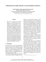
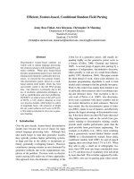
Figure 1: The average running time per iteration against
the average number of senses per correlated words.
two is (with one exception) better than either alone.
As more correlations are added, NA
¨
IVE’s time in-
creases while that of FAST-RB decreases. This is be-
cause the number of non-zero paths for uncorrelated
words decreases as more correlations are added to the
model. Since our techniques save computation for
every zero path, the overall computation decreases
as correlations push uncorrelated words to a limited
number of topics (Figure 1). Qualitatively, when the
synset with “king” and “baron” is added to a model,
it is associated with “drug, inmate, colombia, water-

front, baron” in a topic; when “king” is correlated
with “queen”, the associated topic has “king, parade,
museum, queen, jackson” as its most probable words.
These represent reasonable disambiguations. In con-
trast to previous approaches, inference speeds up as
topics become more semantically coherent (Boyd-
Graber et al., 2007).
6 Conclusion
We demonstrated efficient inference techniques for
topic models with tree-based priors. These methods
scale well, allowing for faster exploration of models
that use semantics to encode correlations without sac-
rificing accuracy. Improved scalability for such algo-
rithms, especially in distributed environments (Smola
and Narayanamurthy, 2010), could improve applica-
tions such as cross-language information retrieval,
unsupervised word sense disambiguation, and knowl-
edge discovery via interactive topic modeling.
278
Acknowledgments
We would like to thank David Mimno and the anony-
mous reviewers for their helpful comments. This
work was supported by the Army Research Labora-
tory through ARL Cooperative Agreement W911NF-
09-2-0072. Any opinions or conclusions expressed
are the authors’ and do not necessarily reflect those
of the sponsors.
References
Steven Abney and Marc Light. 1999. Hiding a seman-
tic hierarchy in a Markov model. In Proceedings of

the Workshop on Unsupervised Learning in Natural
Language Processing.
David Andrzejewski, Xiaojin Zhu, and Mark Craven.
2009. Incorporating domain knowledge into topic mod-
eling via Dirichlet forest priors. In Proceedings of
International Conference of Machine Learning.
David M. Blei, Andrew Ng, and Michael Jordan. 2003.
Latent Dirichlet allocation. Journal of Machine Learn-
ing Research, 3:993–1022.
Jordan Boyd-Graber, David M. Blei, and Xiaojin Zhu.
2007. A topic model for word sense disambiguation.
In Proceedings of Emperical Methods in Natural Lan-
guage Processing.
Gregor Heinrich. 2004. Parameter estima-
tion for text analysis. Technical report.
/>Yuening Hu, Jordan Boyd-Graber, and Brianna Satinoff.
2011. Interactive topic modeling. In Association for
Computational Linguistics.
Jagadeesh Jagarlamudi and Hal Daum
´
e III. 2010. Ex-
tracting multilingual topics from unaligned corpora. In
Proceedings of the European Conference on Informa-
tion Retrieval (ECIR).
George A. Miller. 1990. Nouns in WordNet: A lexical
inheritance system. International Journal of Lexicog-
raphy, 3(4):245–264.
Alexander J. Smola and Shravan Narayanamurthy. 2010.
An architecture for parallel topic models. International
Conference on Very Large Databases, 3.

Limin Yao, David Mimno, and Andrew McCallum. 2009.
Efficient methods for topic model inference on stream-
ing document collections. In Knowledge Discovery and
Data Mining.
279