Báo cáo khoa học: "Regular tree grammars as a formalism for scope underspecification" docx
Bạn đang xem bản rút gọn của tài liệu. Xem và tải ngay bản đầy đủ của tài liệu tại đây (222.17 KB, 9 trang )
Proceedings of ACL-08: HLT, pages 218–226,
Columbus, Ohio, USA, June 2008.
c
2008 Association for Computational Linguistics
Regular tree grammars as a formalism for scope underspecification
Alexander Koller
∗
∗
University of Edinburgh
Michaela Regneri
† §
†
University of Groningen
Stefan Thater
§
§
Saarland University
Abstract
We propose the use of regular tree grammars
(RTGs) as a formalism for the underspecified
processing of scope ambiguities. By applying
standard results on RTGs, we obtain a novel
algorithm for eliminating equivalent readings
and the first efficient algorithm for computing
the best reading of a scope ambiguity. We also
show how to derive RTGs from more tradi-
tional underspecified descriptions.
1 Introduction
Underspecification (Reyle, 1993; Copestake et al.,
2005; Bos, 1996; Egg et al., 2001) has become the
standard approach to dealing with scope ambiguity
in large-scale hand-written grammars (see e.g. Cope-
stake and Flickinger (2000)). The key idea behind
underspecification is that the parser avoids comput-
ing all scope readings. Instead, it computes a single
compact underspecified description for each parse.
One can then strengthen the underspecified descrip-
tion to efficiently eliminate subsets of readings that
were not intended in the given context (Koller and
Niehren, 2000; Koller and Thater, 2006); so when
the individual readings are eventually computed, the
number of remaining readings is much smaller and
much closer to the actual perceived ambiguity of the
sentence.
In the past few years, a “standard model” of scope
underspecification has emerged: A range of for-
malisms from Underspecified DRT (Reyle, 1993)
to dominance graphs (Althaus et al., 2003) have
offered mechanisms to specify the “semantic mate-
rial” of which the semantic representations are built
up, plus dominance or outscoping relations between
these building blocks. This has been a very suc-
cessful approach, but recent algorithms for elimi-
nating subsets of readings have pushed the expres-
sive power of these formalisms to their limits; for
instance, Koller and Thater (2006) speculate that
further improvements over their (incomplete) redun-
dancy elimination algorithm require a more expres-
sive formalism than dominance graphs. On the theo-
retical side, Ebert (2005) has shown that none of
the major underspecification formalisms are expres-
sively complete, i.e. supports the description of an
arbitrary subset of readings. Furthermore, the some-
what implicit nature of dominance-based descrip-
tions makes it difficult to systematically associate
readings with probabilities or costs and then com-
pute a best reading.
In this paper, we address both of these shortcom-
ings by proposing regular tree grammars (RTGs)
as a novel underspecification formalism. Regular
tree grammars (Comon et al., 2007) are a standard
approach for specifying sets of trees in theoretical
computer science, and are closely related to regu-
lar tree transducers as used e.g. in recent work on
statistical MT (Knight and Graehl, 2005) and gram-
mar formalisms (Shieber, 2006). We show that the
“dominance charts” proposed by Koller and Thater
(2005b) can be naturally seen as regular tree gram-
mars; using their algorithm, classical underspecified
descriptions (dominance graphs) can be translated
into RTGs that describe the same sets of readings.
However, RTGs are trivially expressively complete
because every finite tree language is also regular. We
exploit this increase in expressive power in present-
ing a novel redundancy elimination algorithm that is
simpler and more powerful than the one by Koller
and Thater (2006); in our algorithm, redundancy
elimination amounts to intersection of regular tree
languages. Furthermore, we show how to define a
PCFG-style cost model on RTGs and compute best
readings of deterministic RTGs efficiently, and illus-
trate this model on a machine learning based model
218
of scope preferences (Higgins and Sadock, 2003).
To our knowledge, this is the first efficient algorithm
for computing best readings of a scope ambiguity in
the literature.
The paper is structured as follows. In Section 2,
we will first sketch the existing standard approach
to underspecification. We will then define regular
tree grammars and show how to see them as an un-
derspecification formalism in Section 3. We will
present the new redundancy elimination algorithm,
based on language intersection, in Section 4, and
show how to equip RTGs with weights and compute
best readings in Section 5. We conclude in Section 6.
2 Underspecification
The key idea behind scope underspecification is to
describe all readings of an ambiguous expression
with a single, compact underspecified representation
(USR). This simplifies semantics construction, and
current algorithms (Koller and Thater, 2005a) sup-
port the efficient enumeration of readings from an
USR when it is necessary. Furthermore, it is possible
to perform certain semantic processing tasks such
as eliminating redundant readings (see Section 4) di-
rectly on the level of underspecified representations
without explicitly enumerating individual readings.
Under the “standard model” of scope underspeci-
fication, readings are considered as formulas or trees.
USRs specify the “semantic material” common to
all readings, plus dominance or outscopes relations
between these building blocks. In this paper, we con-
sider dominance graphs (Egg et al., 2001; Althaus
et al., 2003) as one representative of this class. An
example dominance graph is shown on the left of
Fig. 1. It represents the five readings of the sentence
“a representative of a company saw every sample.”
The (directed, labelled) graph consists of seven sub-
trees, or fragments, plus dominance edges relating
nodes of these fragments. Each reading is encoded
as one configuration of the dominance graph, which
can be obtained by “plugging” the tree fragments
into each other, in a way that respects the dominance
edges: The source node of each dominance edge
must dominate (i.e., be an ancestor of) the target
node in each configuration. The trees in Fig. 1a–e
are the five configurations of the example graph.
An important class of dominance graphs are hy-
pernormally connected dominance graphs, or dom-
inance nets (Niehren and Thater, 2003). The pre-
cise definition of dominance nets is not important
here, but note that virtually all underspecified de-
scriptions that are produced by current grammars are
nets (Flickinger et al., 2005). For the rest of the pa-
per, we restrict ourselves to dominance graphs that
are hypernormally connected.
3 Regular tree grammars
We will now recall the definition of regular tree
grammars and show how they can be used as an un-
derspecification formalism.
3.1 Definition
Let Σ be an alphabet, or signature, of tree construc-
tors { f ,g, a, .}, each of which is equipped with an
arity ar( f ) ≥ 0. A finite constructor tree t is a finite
tree in which each node is labelled with a symbol of
Σ, and the number of children of the node is exactly
the arity of this symbol. For instance, the configura-
tions in Fig. 1a-e are finite constructor trees over the
signature {a
x
|2, a
y
|2, comp
z
|0, . }. Finite construc-
tor trees can be seen as ground terms over Σ that
respect the arities. We write T (Σ) for the finite con-
structor trees over Σ.
A regular tree grammar (RTG) is a 4-tuple G =
(S, N, Σ, R) consisting of a nonterminal alphabet N,
a terminal alphabet Σ, a start symbol S ∈ N, and a
finite set of production rules R of the form A → β ,
where A ∈ N and β ∈ T (Σ ∪ N); the nonterminals
count as zero-place constructors. Two finite con-
structor trees t,t
∈ T (Σ ∪ N) stand in the deriva-
tion relation, t →
G
t
, if t
can be built from t by
replacing an occurrence of some nonterminal A by
the tree on the right-hand side of some production
for A. The language generated by G, L(G), is the set
{t ∈ T (Σ) | S →
∗
G
t}, i.e. all terms of terminal sym-
bols that can be derived from the start symbol by a
sequence of rule applications. Note that L(G) is a
possibly infinite language of finite trees. As usual,
we write A → t
1
| . . . | t
n
as shorthand for the n pro-
duction rules A → t
i
(1 ≤ i ≤ n). See Comon et al.
(2007) for more details.
The languages that can be accepted by regular tree
grammars are called regular tree languages (RTLs),
and regular tree grammars are equivalent to regular
219
every
y
sample
y
see
x,y
a
x
repr-of
x,z
a
z
comp
z
12 3
4 5 6
7
every
y
a
x
sample
y
see
x,y
repr-of
x,z
a
z
comp
z
(a)
every
y
a
z
a
x
sample
y
see
x,y
comp
z
repr-of
x,z
(c)
every
y
a
z
a
x
sample
y
see
x,y
comp
z
repr-of
x,z
(d)(b)
every
y
sample
y
see
x,y
a
x
repr-of
x,z
a
z
comp
z
(e)
every
y
sample
y
a
x
repr-of
x,z
see
x,y
a
z
comp
z
Figure 1: A dominance graph (left) and its five configurations.
tree automata, which are defined essentially like the
well-known regular string automata, except that they
assign states to the nodes in a tree rather than the po-
sitions in a string. Tree automata are related to tree
transducers as used e.g. in statistical machine trans-
lation (Knight and Graehl, 2005) exactly like finite-
state string automata are related to finite-state string
transducers, i.e. they use identical mechanisms to ac-
cept rather than transduce languages. Many theoreti-
cal results carry over from regular string languages
to regular tree languages; for instance, membership
of a tree in a RTL can be decided in linear time,
RTLs are closed under intersection, union, and com-
plement, and so forth.
3.2 Regular tree grammars in
underspecification
We can now use regular tree grammars in underspeci-
fication by representing the semantic representations
as trees and taking an RTG G as an underspecified
description of the trees in L(G). For example, the
five configurations in Fig. 1 can be represented as
the tree language accepted by the following gram-
mar with start symbol S.
S → a
x
(A
1
, A
2
) | a
z
(B
1
, A
3
) | every
y
(B
3
, A
4
)
A
1
→ a
z
(B
1
, B
2
)
A
2
→ every
y
(B
3
, B
4
)
A
3
→ a
x
(B
2
, A
2
) | every
y
(B
3
, A
5
)
A
4
→ a
x
(A
1
, B
4
) | a
z
(B
1
, A
5
)
A
5
→ a
x
(B
2
, B
4
)
B
1
→ comp
z
B
2
→ repr-of
x,z
B
3
→ sample
y
B
4
→ see
x,y
More generally, every finite set of trees can be
written as the tree language accepted by a non-
recursive regular tree grammar such as this. This
grammar can be much smaller than the set of trees,
because nonterminal symbols (which stand for sets
of possibly many subtrees) can be used on the right-
hand sides of multiple rules. Thus an RTG is a com-
pact representation of a set of trees in the same way
that a parse chart is a compact representation of the
set of parse trees of a context-free string grammar.
Note that each tree can be enumerated from the RTG
in linear time.
3.3 From dominance graphs to tree grammars
Furthermore, regular tree grammars can be system-
atically computed from more traditional underspeci-
fied descriptions. Koller and Thater (2005b) demon-
strate how to compute a dominance chart from a
dominance graph D by tabulating how a subgraph
can be decomposed into smaller subgraphs by re-
moving what they call a “free fragment”. If D is
hypernormally connected, this chart can be read as
a regular tree grammar whose nonterminal symbols
are subgraphs of the dominance graph, and whose
terminal symbols are names of fragments. For the
example graph in Fig. 1, it looks as follows.
{1, 2, 3, 4, 5, 6, 7} → 1({2, 4, 5}, {3, 6, 7})
{1, 2, 3, 4, 5, 6, 7} → 2({4}, {1, 3, 5, 6, 7})
{1, 2, 3, 4, 5, 6, 7} → 3({6}, {1, 2, 4, 5, 7})
{1, 3, 5, 6, 7} → 1({5}, {3, 6, 7}) | 3({6}, {1, 5, 7})
{1, 2, 4, 5, 7} → 1({2, 4, 5}, {7}) | 2({4}, {1, 5, 7})
{1, 5, 7} → 1({5}, {7})
{2, 4, 5} → 2({4}, {5}) {4} → 4 {6} → 6
{3, 6, 7} → 3({6}, {7}) {5} → 5 {7} → 7
This grammar accepts, again, five different trees,
whose labels are the node names of the dominance
graph, for instance 1(2(4, 5), 3(6, 7)). If f : Σ → Σ
is a relabelling function from one terminal alpha-
bet to another, we can write f (G) for the grammar
(S, N, Σ
, R
), where R
= {A → f (a)(B
1
, . , B
n
) |
A → a(B
1
, . , B
n
) ∈ R}. Now if we choose f to be
the labelling function of D (which maps node names
to node labels) and G is the chart of D, then L( f (G))
will be the set of configurations of D. The grammar
in Section 3.2 is simply f (G) for the chart above (up
to consistent renaming of nonterminals).
In the worst case, the dominance chart of a dom-
inance graph with n fragments has O(2
n
) produc-
tion rules (Koller and Thater, 2005b), i.e. charts may
be exponential in size; but note that this is still an
220
1,0E+00
1,0E+04
1,0E+08
1,0E+12
1,0E+16
1 3 5 7 9 11 13 15 17 19 21 23 25 27 29 31 33
#fragments
#configurations/rules
0
10
20
30
40
50
60
70
80
#sentences
#sentences
#production rules in chart
#configurations
Figure 2: Chart sizes in the Rondane corpus.
improvement over the n! configurations that these
worst-case examples have. In practice, RTGs that
are computed by converting the USR computed by a
grammar remain compact: Fig. 2 compares the aver-
age number of configurations and the average num-
ber of RTG production rules for USRs of increasing
sizes in the Rondane treebank (see Sect. 4.3); the
bars represent the number of sentences for USRs of a
certain size. Even for the most ambiguous sentence,
which has about 4.5 ×10
12
scope readings, the domi-
nance chart has only about 75 000 rules, and it takes
only 15 seconds on a modern consumer PC (Intel
Core 2 Duo at 2 GHz) to compute the grammar from
the graph. Computing the charts for all 999 MRS-
nets in the treebank takes about 45 seconds.
4 Expressive completeness and
redundancy elimination
Because every finite tree language is regular, RTGs
constitute an expressively complete underspecifica-
tion formalism in the sense of Ebert (2005): They
can represent arbitrary subsets of the original set of
readings. Ebert shows that the classical dominance-
based underspecification formalisms, such as MRS,
Hole Semantics, and dominance graphs, are all
expressively incomplete, which Koller and Thater
(2006) speculate might be a practical problem for al-
gorithms that strengthen USRs to remove unwanted
readings. We will now show how both the expres-
sive completeness and the availability of standard
constructions for RTGs can be exploited to get an
improved redundancy elimination algorithm.
4.1 Redundancy elimination
Redundancy elimination (Vestre, 1991; Chaves,
2003; Koller and Thater, 2006) is the problem of de-
riving from an USR U another USR U
, such that
the readings of U
are a proper subset of the read-
ings of U, but every reading in U is semantically
equivalent to some reading in U
. For instance, the
following sentence from the Rondane treebank is an-
alyzed as having six quantifiers and 480 readings by
the ERG grammar; these readings fall into just two
semantic equivalence classes, characterized by the
relative scope of “the lee of” and “a small hillside”.
A redundancy elimination would therefore ideally re-
duce the underspecified description to one that has
only two readings (one for each class).
(1) We quickly put up the tents in the lee of a
small hillside and cook for the first time in the
open. (Rondane 892)
Koller and Thater (2006) define semantic equiva-
lence in terms of a rewrite system that specifies un-
der what conditions two quantifiers may exchange
their positions without changing the meaning of the
semantic representation. For example, if we assume
the following rewrite system (with just a single rule),
the five configurations in Fig. 1a-e fall into three
equivalence classes – indicated by the dotted boxes
around the names a-e – because two pairs of read-
ings can be rewritten into each other.
(2) a
x
(a
z
(P, Q), R) → a
z
(P, a
x
(Q, R))
Based on this definition, Koller and Thater (2006)
present an algorithm (henceforth, KT06) that deletes
rules from a dominance chart and thus removes sub-
sets of readings from the USR. The KT06 algorithm
is fast and quite effective in practice. However, it es-
sentially predicts for each production rule of a dom-
inance chart whether each configuration that can be
built with this rule is equivalent to a configuration
that can be built with some other production for the
same subgraph, and is therefore rather complex.
4.2 Redundancy elimination as language
intersection
We now define a new algorithm for redundancy elim-
ination. It is based on the intersection of regular tree
languages, and will be much simpler and more pow-
erful than KT06.
Let G = (S, N, Σ, R) be an RTG with a linear or-
der on the terminals Σ; for ease of presentation, we
assume Σ ⊆ N. Furthermore, let f : Σ → Σ
be a re-
labelling function into the signature Σ
of the rewrite
221
system. For example, G could be the dominance
chart of some dominance graph D, and f could be
the labelling function of D.
We can then define a tree language L
F
as follows:
L
F
contains all trees over Σ that do not contain a sub-
tree of the form q
1
(x
1
, . . . , x
i−1
, q
2
(. . .), x
i+1
, . . . , x
k
)
where q
1
> q
2
and the rewrite system contains a rule
that has f (q
1
)(X
1
, . . . , X
i−1
, f (q
2
)(. . .), X
i+1
, . . . , X
k
)
on the left or right hand side. L
F
is a regular tree lan-
guage, and can be accepted by a regular tree gram-
mar G
F
with O(n) nonterminals and O(n
2
) rules,
where n = |Σ
|. A filter grammar for Fig. 1 looks
as follows:
S → 1(S, S) | 2(S, Q
1
) | 3(S, S) | 4 | . | 7
Q
1
→ 2(S, Q
1
) | 3(S, S) | 4 | . | 7
This grammar accepts all trees over Σ except ones
in which a node with label 2 is the parent of a node
with label 1, because such trees correspond to config-
urations in which a node with label a
z
is the parent of
a node with label a
x
, a
z
and a
x
are permutable, and
2 > 1. In particular, it will accept the configurations
(b), (c), and (e) in Fig. 1, but not (a) or (d).
Since regular tree languages are closed under in-
tersection, we can compute a grammar G
such that
L(G
) = L(G)∩L
F
. This grammar has O(nk) nonter-
minals and O(n
2
k) productions, where k is the num-
ber of production rules in G, and can be computed
in time O(n
2
k). The relabelled grammar f (G
) ac-
cepts all trees in which adjacent occurrences of per-
mutable quantifiers are in a canonical order (sorted
from lowest to highest node name). For example, the
grammar G
for the example looks as follows; note
that the nonterminal alphabet of G
is the product of
the nonterminal alphabets of G and G
F
.
{1, 2, 3, 4, 5, 6, 7}
S
→ 1({2, 4, 5}
S
, {3, 6, 7}
S
)
{1, 2, 3, 4, 5, 6, 7}
S
→ 2({4}
S
, {1, 3, 5, 6, 7}
Q
1
)
{1, 2, 3, 4, 5, 6, 7}
S
→ 3({6}
S
, {1, 2, 4, 5, 7}
S
)
{1, 3, 5, 6, 7}
Q
1
→ 3({6}
S
, {1, 5, 7}
S
)
{1, 2, 4, 5, 7}
S
→ 1({2, 4, 5}
S
, {7}
S
)
{1, 2, 4, 5, 7}
S
→ 2({4}
S
, {1, 5, 7}
Q
1
)
{2, 4, 5}
S
→ 2({4}
S
, {5}
Q
1
) {4}
S
→ 4
{3, 6, 7}
S
→ 3({6}
S
, {7}
S
) {5}
S
→ 5
{1, 5, 7}
S
→ 1({5}
S
, {7}
S
) {5}
Q
1
→ 5
{6}
S
→ 6 {7}
S
→ 7
Significantly, the grammar contains no produc-
tions for {1, 3, 5, 6, 7}
Q
1
with terminal symbol 1, and
no production for {1, 5, 7}
Q
1
. This reduces the tree
language accepted by f (G
) to just the configura-
tions (b), (c), and (e) in Fig. 1, i.e. exactly one
representative of every equivalence class. Notice
that there are two different nonterminals, {5}
Q
1
and
{5}
S
, corresponding to the subgraph {5}, so the in-
tersected RTG is not a dominance chart any more.
As we will see below, this increased expressivity in-
creases the power of the redundancy elimination al-
gorithm.
4.3 Evaluation
The algorithm presented here is not only more trans-
parent than KT06, but also more powerful; for exam-
ple, it will reduce the graph in Fig. 4 of Koller and
Thater (2006) completely, whereas KT06 won’t.
To measure the extent to which the new algo-
rithm improves upon KT06, we compare both algo-
rithms on the USRs in the Rondane treebank (ver-
sion of January 2006). The Rondane treebank is a
“Redwoods style” treebank (Oepen et al., 2002) con-
taining MRS-based underspecified representations
for sentences from the tourism domain, and is dis-
tributed together with the English Resource Gram-
mar (ERG) (Copestake and Flickinger, 2000).
The treebank contains 999 MRS-nets, which we
translate automatically into dominance graphs and
further into RTGs; the median number of scope read-
ings per sentence is 56. For our experiment, we con-
sider all 950 MRS-nets with less than 650 000 con-
figurations. We use a slightly weaker version of the
rewrite system that Koller and Thater (2006) used in
their evaluation.
It turns out that the median number of equivalence
classes, computed by pairwise comparison of all con-
figurations, is 8. The median number of configu-
rations that remain after running our algorithm is
also 8. By contrast, the median number after run-
ning KT06 is 11. For a more fine-grained compari-
son, Fig. 3 shows the percentage of USRs for which
the two algorithms achieve complete reduction, i.e.
retain only one reading per equivalence class. In the
diagram, we have grouped USRs according to the
natural logarithm of their numbers of configurations,
and report the percentage of USRs in this group on
which the algorithms were complete. The new algo-
rithm dramatically outperforms KT06: In total, it re-
duces 96% of all USRs completely, whereas KT06
was complete only for 40%. This increase in com-
pleteness is partially due to the new algorithm’s abil-
ity to use non-chart RTGs: For 28% of the sentences,
222
0%
20%
40%
60%
80%
100%
1 3 5 7 9 11 13
KT06 RTG
Figure 3: Percentage of USRs in Rondane for which the
algorithms achieve complete reduction.
it computes RTGs that are not dominance charts.
KT06 was only able to reduce 5 of these 263 graphs
completely.
The algorithm needs 25 seconds to run for the
entire corpus (old algorithm: 17 seconds), and it
would take 50 (38) more seconds to run on the 49
large USRs that we exclude from the experiment.
By contrast, it takes about 7 hours to compute the
equivalence classes by pairwise comparison, and it
would take an estimated several billion years to com-
pute the equivalence classes of the excluded USRs.
In short, the redundancy elimination algorithm pre-
sented here achieves nearly complete reduction at a
tiny fraction of the runtime, and makes a useful task
that was completely infeasible before possible.
4.4 Compactness
Finally, let us briefly consider the ramifications of
expressive completeness on efficiency. Ebert (2005)
proves that no expressively complete underspecifi-
cation formalism can be compact, i.e. in the worst
case, the USR of a set of readings become exponen-
tially large in the number of scope-bearing operators.
In the case of RTGs, this worst case is achieved by
grammars of the form S → t
1
| . . . | t
n
, where t
1
, . . . , t
n
are the trees we want to describe. This grammar is as
big as the number of readings, i.e. worst-case expo-
nential in the number n of scope-bearing operators,
and essentially amounts to a meta-level disjunction
over the readings.
Ebert takes the incompatibility between compact-
ness and expressive completeness as a fundamental
problem for underspecification. We don’t see things
quite as bleakly. Expressions of natural language it-
self are (extremely underspecified) descriptions of
sets of semantic representations, and so Ebert’s ar-
gument applies to NL expressions as well. This
means that describing a given set of readings may
require an exponentially long discourse. Ebert’s def-
inition of compactness may be too harsh: An USR,
although exponential-size in the number of quanti-
fiers, may still be polynomial-size in the length of
the discourse in the worst case.
Nevertheless, the tradeoff between compactness
and expressive power is important for the design
of underspecification formalisms, and RTGs offer a
unique answer. They are expressively complete; but
as we have seen in Fig. 2, the RTGs that are derived
by semantic construction are compact, and even in-
tersecting them with filter grammars for redundancy
elimination only blows up their sizes by a factor of
O(n
2
). As we add more and more information to
an RTG to reduce the set of readings, ultimately to
those readings that were meant in the actual context
of the utterance, the grammar will become less and
less compact; but this trend is counterbalanced by
the overall reduction in the number of readings. For
the USRs in Rondane, the intersected RTGs are, on
average, 6% smaller than the original charts. Only
30% are larger than the charts, by a maximal factor
of 3.66. Therefore we believe that the theoretical
non-compactness should not be a major problem in
a well-designed practical system.
5 Computing best configurations
A second advantage of using RTGs as an under-
specification formalism is that we can apply exist-
ing algorithms for computing the best derivations
of weighted regular tree grammars to compute best
(that is, cheapest or most probable) configurations.
This gives us the first efficient algorithm for comput-
ing the preferred reading of a scope ambiguity.
We define weighted dominance graphs and
weighted tree grammars, show how to translate the
former into the latter and discuss an example.
5.1 Weighted dominance graphs
A weighted dominance graph D = (V, E
T
E
D
W
D
W
I
) is a dominance graph with two new types
of edges – soft dominance edges, W
D
, and soft dis-
jointness edges, W
I
–, each of which is equipped
with a numeric weight. Soft dominance and dis-
jointness edges provide a mechanism for assigning
weights to configurations; a soft dominance edge ex-
223
every
y
sample
y
see
x,y
a
x
repr-of
x,z
a
z
comp
z
1
2
3
4 5 6
7
9
8
Figure 4: The graph of Fig. 1 with soft constraints
presses a preference that two nodes dominate each
other in a configuration, whereas a soft disjointness
edge expresses a preference that two nodes are dis-
joint, i.e. neither dominates the other.
We take the hard backbone of D to be the ordinary
dominance graph B(D) = (V, E
T
E
D
) obtained by
removing all soft edges. The set of configurations
of a weighted graph D is the set of configurations
of its hard backbone. For each configuration t of
D, we define the weight c(t) to be the product of
the weights of all soft dominance and disjointness
edges that are satisfied in t. We can then ask for
configurations of maximal weight.
Weighted dominance graphs can be used to en-
code the standard models of scope preferences
(Pafel, 1997; Higgins and Sadock, 2003). For exam-
ple, Higgins and Sadock (2003) present a machine
learning approach for determining pairwise prefer-
ences as to whether a quantifier Q
1
dominates an-
other quantifier Q
2
, Q
2
dominates Q
1
, or neither (i.e.
they are disjoint). We can represent these numbers
as the weights of soft dominance and disjointness
edges. An example (with artificial weights) is shown
in Fig. 4; we draw the soft dominance edges as
curved dotted arrows and the soft disjointness edges
as as angled double-headed arrows. Each soft edge
is annotated with its weight. The hard backbone
of this dominance graph is our example graph from
Fig. 1, so it has the same five configurations. The
weighted graph assigns a weight of 8 to configura-
tion (a), a weight of 1 to (d), and a weight of 9 to (e);
this is also the configuration of maximum weight.
5.2 Weighted tree grammars
In order to compute the maximal-weight configura-
tion of a weighted dominance graph, we will first
translate it into a weighted regular tree grammar. A
weighted regular tree grammar (wRTG) (Graehl and
Knight, 2004) is a 5-tuple G = (S, N, Σ, R, c) such
that G
= (S, N, Σ, R) is a regular tree grammar and
c : R → R is a function that assigns each production
rule a weight. G accepts the same language of trees
as G
. It assigns each derivation a cost equal to the
product of the costs of the production rules used in
this derivation, and it assigns each tree in the lan-
guage a cost equal to the sum of the costs of its
derivations. Thus wRTGs define weights in a way
that is extremely similar to PCFGs, except that we
don’t require any weights to sum to one.
Given a weighted, hypernormally connected dom-
inance graph D, we can extend the chart of B(D) to
a wRTG by assigning rule weights as follows: The
weight of a rule D
0
→ i(D
1
, . . . , D
n
) is the product
over the weights of all soft dominance and disjoint-
ness edges that are established by this rule. We say
that a rule establishes a soft dominance edge from
u to v if u = i and v is in one of the subgraphs
D
1
, . . . , D
n
; we say that it establishes a soft disjoint-
ness edge between u and v if u and v are in different
subgraphs D
j
and D
k
( j = k). It can be shown that
the weight this grammar assigns to each derivation
is equal to the weight that the original dominance
graph assigns to the corresponding configuration.
If we apply this construction to the example graph
in Fig. 4, we obtain the following wRTG:
{1, , 7} → a
x
({2, 4, 5}, {3, 6, 7}) [9]
{1, , 7} → a
z
({4}, {1, 3, 5, 6, 7}) [1]
{1, , 7} → every
y
({6}, {1, 2, 4, 5, 7}) [8]
{2, 4, 5} → a
z
({4}, {5}) [1]
{3, 6, 7} → every
y
({6}, {7}) [1]
{1, 3, 5, 6, 7} → a
x
({5}, {3, 6, 7}) [1]
{1, 3, 5, 6, 7} → every
y
({6}, {1, 5, 7}) [8]
{1, 2, 4, 5, 7} → a
x
({2, 4, 5}, {7}) [1]
{1, 2, 4, 5, 7} → a
z
({4}, {1, 5, 7}) [1]
{1, 5, 7} → a
x
({5}, {7}) [1]
{4} → comp
z
[1] {5} → repr−o f
x,z
[1]
{6} → sample
y
[1] {7} → see
x,y
[1]
For example, picking “a
z
” as the root of a con-
figuration (Fig. 1 (c), (d)) of the entire graph has
a weight of 1, because this rule establishes no soft
edges. On the other hand, choosing “a
x
” as the root
has a weight of 9, because this establishes the soft
disjointness edge (and in fact, leads to the derivation
of the maximum-weight configuration in Fig. 1 (e)).
5.3 Computing the best configuration
The problem of computing the best configuration of
a weighted dominance graph – or equivalently, the
224
best derivation of a weighted tree grammar – can
now be solved by standard algorithms for wRTGs.
For example, Knight and Graehl (2005) present an
algorithm to extract the best derivation of a wRTG in
time O(t + nlog n) where n is the number of nonter-
minals and t is the number of rules. In practice, we
can extract the best reading of the most ambiguous
sentence in the Rondane treebank (4.5 × 10
12
read-
ings, 75 000 grammar rules) with random soft edges
in about a second.
However, notice that this is not the same problem
as computing the best tree in the language accepted
by a wRTG, as trees may have multiple deriva-
tions. The problem of computing the best tree is NP-
complete (Sima’an, 1996). However, if the weighted
regular tree automaton corresponding to the wRTG
is deterministic, every tree has only one derivation,
and thus computing best trees becomes easy again.
The tree automata for dominance charts are always
deterministic, and the automata for RTGs as in Sec-
tion 3.2 (whose terminals correspond to the graph’s
node labels) are also typically deterministic if the
variable names are part of the quantifier node labels.
Furthermore, there are algorithms for determinizing
weighted tree automata (Borchardt and Vogler, 2003;
May and Knight, 2006), which could be applied as
preprocessing steps for wRTGs.
6 Conclusion
In this paper, we have shown how regular tree gram-
mars can be used as a formalism for scope under-
specification, and have exploited the power of this
view in a novel, simpler, and more complete algo-
rithm for redundancy elimination and the first effi-
cient algorithm for computing the best reading of a
scope ambiguity. In both cases, we have adapted
standard algorithms for RTGs, which illustrates the
usefulness of using such a well-understood formal-
ism. In the worst case, the RTG for a scope ambigu-
ity is exponential in the number of scope bearers in
the sentence; this is a necessary consequence of their
expressive completeness. However, those RTGs that
are computed by semantic construction and redun-
dancy elimination remain compact.
Rather than showing how to do semantic construc-
tion for RTGs, we have presented an algorithm that
computes RTGs from more standard underspecifica-
tion formalisms. We see RTGs as an “underspecifi-
cation assembly language” – they support efficient
and useful algorithms, but direct semantic construc-
tion may be inconvenient, and RTGs will rather be
obtained by “compiling” higher-level underspecified
representations such as dominance graphs or MRS.
This perspective also allows us to establish a
connection to approaches to semantic construc-
tion which use chart-based packing methods rather
than dominance-based underspecification to manage
scope ambiguities. For instance, both Combinatory
Categorial Grammars (Steedman, 2000) and syn-
chronous grammars (Nesson and Shieber, 2006) rep-
resent syntactic and semantic ambiguity as part of
the same parse chart. These parse charts can be
seen as regular tree grammars that accept the lan-
guage of parse trees, and conceivably an RTG that
describes only the semantic and not the syntactic
ambiguity could be automatically extracted. We
could thus reconcile these completely separate ap-
proaches to semantic construction within the same
formal framework, and RTG-based algorithms (e.g.,
for redundancy elimination) would apply equally to
dominance-based and chart-based approaches. In-
deed, for one particular grammar formalism it has
even been shown that the parse chart contains an
isomorphic image of a dominance chart (Koller and
Rambow, 2007).
Finally, we have only scratched the surface of
what can be be done with the computation of best
configurations in Section 5. The algorithms gen-
eralize easily to weights that are taken from an ar-
bitrary ordered semiring (Golan, 1999; Borchardt
and Vogler, 2003) and to computing minimal-weight
rather than maximal-weight configurations. It is also
useful in applications beyond semantic construction,
e.g. in discourse parsing (Regneri et al., 2008).
Acknowledgments. We have benefited greatly
from fruitful discussions on weighted tree grammars
with Kevin Knight and Jonathan Graehl, and on dis-
course underspecification with Markus Egg. We
also thank Christian Ebert, Marco Kuhlmann, Alex
Lascarides, and the reviewers for their comments on
the paper. Finally, we are deeply grateful to our for-
mer colleague Joachim Niehren, who was a great fan
of tree automata before we even knew what they are.
225
References
E. Althaus, D. Duchier, A. Koller, K. Mehlhorn,
J. Niehren, and S. Thiel. 2003. An efficient graph
algorithm for dominance constraints. J. Algorithms,
48:194–219.
B. Borchardt and H. Vogler. 2003. Determinization of
finite state weighted tree automata. Journal of Au-
tomata, Languages and Combinatorics, 8(3):417–463.
J. Bos. 1996. Predicate logic unplugged. In Proceedings
of the Tenth Amsterdam Colloquium, pages 133–143.
R. P. Chaves. 2003. Non-redundant scope disambigua-
tion in underspecified semantics. In Proceedings of
the 8th ESSLLI Student Session, pages 47–58, Vienna.
H. Comon, M. Dauchet, R. Gilleron, C. L
¨
oding,
F. Jacquemard, D. Lugiez, S. Tison, and M. Tommasi.
2007. Tree automata techniques and applications.
Available on: />A. Copestake and D. Flickinger. 2000. An open-
source grammar development environment and broad-
coverage English grammar using HPSG. In Confer-
ence on Language Resources and Evaluation.
A. Copestake, D. Flickinger, C. Pollard, and I. Sag. 2005.
Minimal recursion semantics: An introduction. Re-
search on Language and Computation, 3:281–332.
C. Ebert. 2005. Formal investigations of underspecified
representations. Ph.D. thesis, King’s College, Lon-
don.
M. Egg, A. Koller, and J. Niehren. 2001. The Constraint
Language for Lambda Structures. Logic, Language,
and Information, 10:457–485.
D. Flickinger, A. Koller, and S. Thater. 2005. A new
well-formedness criterion for semantics debugging. In
Proceedings of the 12th HPSG Conference, Lisbon.
J. S. Golan. 1999. Semirings and their applications.
Kluwer, Dordrecht.
J. Graehl and K. Knight. 2004. Training tree transducers.
In HLT-NAACL 2004, Boston.
D. Higgins and J. Sadock. 2003. A machine learning ap-
proach to modeling scope preferences. Computational
Linguistics, 29(1).
K. Knight and J. Graehl. 2005. An overview of proba-
bilistic tree transducers for natural language process-
ing. In Computational linguistics and intelligent text
processing, pages 1–24. Springer.
A. Koller and J. Niehren. 2000. On underspecified
processing of dynamic semantics. In Proceedings of
COLING-2000, Saarbr
¨
ucken.
A. Koller and O. Rambow. 2007. Relating dominance
formalisms. In Proceedings of the 12th Conference on
Formal Grammar, Dublin.
A. Koller and S. Thater. 2005a. Efficient solving and
exploration of scope ambiguities. Proceedings of the
ACL-05 Demo Session.
A. Koller and S. Thater. 2005b. The evolution of dom-
inance constraint solvers. In Proceedings of the ACL-
05 Workshop on Software.
A. Koller and S. Thater. 2006. An improved redundancy
elimination algorithm for underspecified descriptions.
In Proceedings of COLING/ACL-2006, Sydney.
J. May and K. Knight. 2006. A better n-best list: Prac-
tical determinization of weighted finite tree automata.
In Proceedings of HLT-NAACL.
R. Nesson and S. Shieber. 2006. Simpler TAG semantics
through synchronization. In Proceedings of the 11th
Conference on Formal Grammar.
J. Niehren and S. Thater. 2003. Bridging the gap be-
tween underspecification formalisms: Minimal recur-
sion semantics as dominance constraints. In Proceed-
ings of ACL 2003.
S. Oepen, K. Toutanova, S. Shieber, C. Manning,
D. Flickinger, and T. Brants. 2002. The LinGO Red-
woods treebank: Motivation and preliminary applica-
tions. In Proceedings of the 19th International Con-
ference on Computational Linguistics (COLING’02),
pages 1253–1257.
J. Pafel. 1997. Skopus und logische Struktur: Studien
zum Quantorenskopus im Deutschen. Habilitationss-
chrift, Eberhard-Karls-Universit
¨
at T
¨
ubingen.
M. Regneri, M. Egg, and A. Koller. 2008. Efficient pro-
cessing of underspecified discourse representations. In
Proceedings of the 46th Annual Meeting of the Asso-
ciation for Computational Linguistics: Human Lan-
guage Technologies (ACL-08: HLT) – Short Papers,
Columbus, Ohio.
U. Reyle. 1993. Dealing with ambiguities by underspec-
ification: Construction, representation and deduction.
Journal of Semantics, 10(1).
S. Shieber. 2006. Unifying synchronous tree-adjoining
grammars and tree transducers via bimorphisms. In
Proceedings of the 11th Conference of the European
Chapter of the Association for Computational Linguis-
tics (EACL-06), Trento, Italy.
K. Sima’an. 1996. Computational complexity of proba-
bilistic disambiguation by means of tree-grammars. In
Proceedings of the 16th conference on Computational
linguistics, pages 1175–1180, Morristown, NJ, USA.
Association for Computational Linguistics.
M. Steedman. 2000. The syntactic process. MIT Press.
E. Vestre. 1991. An algorithm for generating non-
redundant quantifier scopings. In Proc. of EACL,
pages 251–256, Berlin.
226