Applied Speech and Audio Processing: With MATLAB doc
Bạn đang xem bản rút gọn của tài liệu. Xem và tải ngay bản đầy đủ của tài liệu tại đây (2.66 MB, 218 trang )
This page intentionally left blank
Applied Speech and Audio Processing: With MATLAB Examples
Applied Speech and Audio Processing isaMatlab-based, one-stop resource that
blends speech and hearing research in describing the key techniques of speech and
audio processing.
This practically orientated text provides Matlab examples throughout to illustrate
the concepts discussed and to give the reader hands-on experience with important tech-
niques. Chapters on basic audio processing and the characteristics of speech and hearing
lay the foundations of speech signal processing, which are built upon in subsequent
sections explaining audio handling, coding, compression and analysis techniques. The
final chapter explores a number of advanced topics that use these techniques, including
psychoacoustic modelling, a subject which underpins MP3 and related audio formats.
With its hands-on nature and numerous Matlab examples, this book is ideal for
graduate students and practitioners working with speech or audio systems.
Ian McLoughlin is an Associate Professor in the School of Computer Engineering,
Nanyang Technological University, Singapore. Over the past 20 years he has worked for
industry, government and academia across three continents. His publications and patents
cover speech processing for intelligibility, compression, detection and interpretation,
hearing models for intelligibility in English and Mandarin Chinese, and psychoacoustic
methods for audio steganography.
Applied Speech and
Audio Processing
With MATLAB Examples
IAN MCLOUGHLIN
School of Computer Engineering
Nanyang Technological University
Singapore
CAMBRIDGE UNIVERSITY PRESS
Cambridge, New York, Melbourne, Madrid, Cape Town, Singapore, São Paulo
Cambridge University Press
The Edinburgh Building, Cambridge CB2 8RU, UK
First published in print format
ISBN-13 978-0-521-51954-0
ISBN-13 978-0-511-51654-2
© Cambridge University Press 2009
2009
Information on this title: www.cambrid
g
e.or
g
/9780521519540
This publication is in copyright. Subject to statutory exception and to the
provision of relevant collective licensing agreements, no reproduction of any part
may take place without the written permission of Cambridge University Press.
Cambridge University Press has no responsibility for the persistence or accuracy
of urls for external or third-party internet websites referred to in this publication,
and does not guarantee that any content on such websites is, or will remain,
accurate or appropriate.
Published in the United States of America by Cambridge University Press, New York
www.cambridge.org
eBook
(
EBL
)
hardback
Contents
Preface page vii
Acknowledgements x
1 Introduction 1
1.1 Digital audio 1
1.2 Capturing and converting sound 2
1.3 Sampling 3
1.4 Summary 5
2 Basic audio processing 7
2.1 Handling audio in Matlab 7
2.2 Normalisation 13
2.3 Audio processing 15
2.4 Segmentation 18
2.5 Analysis window sizing 24
2.6 Visualisation 25
2.7 Sound generation 30
2.8 Summary 34
3 Speech 38
3.1 Speech production 38
3.2 Characteristics of speech 41
3.3 Speech understanding 47
3.4 Summary 54
4 Hearing 59
4.1 Physical processes 59
4.2 Psychoacoustics 60
4.3 Amplitude and frequency models 72
4.4 Psychoacoustic processing 74
4.5 Auditory scene analysis 76
4.6 Summary 85
v
vi Contents
5 Speech communications 89
5.1 Quantisation 90
5.2 Parameterisation 95
5.3 Pitch models 117
5.4 Analysis-by-synthesis 122
5.5 Summary 130
6 Audio analysis 135
6.1 Analysis toolkit 136
6.2 Speech analysis and classification 148
6.3 Analysis of other signals 151
6.4 Higher order statistics 155
6.5 Summary 157
7 Advanced topics 160
7.1 Psychoacoustic modelling 160
7.2 Perceptual weighting 168
7.3 Speaker classification 169
7.4 Language classification 172
7.5 Speech recognition 174
7.6 Speech synthesis 180
7.7 Stereo encoding 184
7.8 Formant strengthening and steering 189
7.9 Voice and pitch changer 193
7.10 Summary 198
Index 202
Preface
Speech and hearing are closely linked human abilities. It could be said that human speech
is optimised toward the frequency ranges that we hear best, or perhaps our hearing is
optimised around the frequencies used for speaking. However whichever way we present
the argument, it should be clear to an engineer working with speech transmission and
processing systems that aspects of both speech and hearing must often be considered
together in the field of vocal communications. However, both hearing and speech remain
complex subjects in their own right. Hearing particularly so.
In recent years it has become popular to discuss psychoacoustics in textbooks on both
hearing and speech. Psychoacoustics is a term that links the words psycho and acoustics
together, and although it sounds like a description of an auditory-challenged serial killer,
actually describes the way the mind processes sound. In particular, it is used to highlight
the fact that humans do not always perceive sound in the straightforward ways that
knowledge of the physical characteristics of the sound would suggest.
There was a time when use of this word at a conference would boast of advanced
knowledge, and familiarity with cutting-edge terminology, especially when it could roll
off the tongue naturally. I would imagine speakers, on the night before their keynote
address, standing before the mirror in their hotel rooms practising saying the word
fluently. However these days it is used far too commonly, to describe any aspect of
hearing that is processed nonlinearly by the brain. It was a great temptation to use the
word in the title of this book.
The human speech process, while more clearly understood than the hearing process,
maintains its own subtleties and difficulties, not least through the profusion of human
languages, voices, inflexions, accents and speaking patterns. Speech is an imperfect
auditory communication system linking the meaning wishing to be expressed in one
brain, to the meaning being imparted in another brain. In the speaker’s brain, the meaning
is encoded into a collection of phonemes which are articulated through movements of
several hundred separate muscles spread from the diaphragm, through to the lips. These
produce sounds which travel through free air, may be encoded by something such as
a telephone system, transmitted via a satellite in space half way around the world, and
then recreated in a different environment to travel through free air again to the outer ears
of a listener. Sounds couple through the outer ear, middle ear, inner ear and finally enter
the brain, on either side of the head. A mixture of lower and higher brain functions then,
hopefully, recreate a meaning.
vii
viii Preface
It is little wonder, given the journey of meaning from one brain to another via mech-
anisms of speech and hearing, that we call for both processes to be considered together.
Thus, this book spans both speech and hearing, primarily in the context of the engineering
of speech communications systems. However, in recognition of the dynamic research
being undertaken in these fields, other areas are also drawn into our discussions: music,
perception of non-speech signals, auditory scene analysis, some unusual hearing effects
and even analysis of birdsong are described.
It is sincerely hoped that through the discussions, and the examples, the reader will
learn to enjoy the analysis and processing of speech and other sounds, and appreciate
the joy of discovering the complexities of the human hearing system.
In orientation, this book is unashamedly practical. It does not labour long over complex
proofs, nor over tedious background theory, which can readily be obtained elsewhere.
It does, wherever possible, provide practical and working examples using Matlab to
illustrate its points. This aims to encourage a culture of experimentation and practical
enquiry in the reader, and to build an enthusiasm for exploration and discovery. Readers
wishing to delve deeper into any of the techniques described will find references to
scientific papers provided in the text, and a bibliography for further reading following
each chapter.
Although few good textbooks currently cover both speech and hearing, there are sev-
eral examples which should be mentioned at this point, along with several narrower
texts. Firstly, the excellent books by Brian Moore of Cambridge University, covering
the psychology of hearing, are both interesting and informative to anyone who is in-
terested in the human auditory system. Several texts by Eberhard Zwicker and Karl D.
Kryter are also excellent references, mainly related to hearing, although Zwicker does
foray occasionally into the world of speech. For a signal processing focus, the extensive
Gold and Morgan text, covering almost every aspect of speech and hearing, is a good
reference.
Overview of the book
In this book I attempt to cover both speech and hearing to a depth required by a fresh post-
graduate student, or an industrial developer, embarking on speech or hearing research.
A basic background of digital signal processing is assumed: for example knowledge of
the Fourier transform and some exposure to discrete digital filtering. This is not a signal
processing text – it is a book that unveils aspects of the arcane world of speech and audio
processing, and does so with Matlab examples where possible. In the process, some
of the more useful techniques in the toolkit of the audio and speech engineer will be
presented.
The motivation for writing this book derives from the generations of students that
I have trained in these fields, almost each of whom required me to cover these same
steps in much the same order, year after year. Typical undergraduate courses in elec-
tronic and/or computer engineering, although they adequately provide the necessary
foundational skills, generally fail to prepare graduates for work in the speech and audio
Preface
ix
signal processing field. The coverage in this book is targeted toward filling the gap. It is
designed to educate, interest and motivate researchers working in this field to build their
skills and capabilities to prepare for research and development in the speech and audio
fields.
This book contains seven chapters that generally delve into deeper and more advanced
topics as the book progresses. Chapter 2 is an introductory background to basic audio
processing and handling in Matlab, and is recommended to those new to using Matlab
for audio work. It also contains justifications for, and explanations of, segmentation,
overlap and windowing, which are fundamental techniques in splitting up and handling
long recordings of speech and audio.
Chapter 3 describes speech production, characteristics, understanding and handling,
followed by Chapter 4 which repeats the same for hearing. Chapter 5 is concerned with
the handling of audio, primarily speech, and Chapter 6 with analysis methods for speech
and audio. Finally Chapter 7 presents some advanced topics that make use of many of
the techniques in earlier chapters.
Arrangement of the book
Each section begins with introductory text explaining the points to be made in the section,
before further detail, and usually Matlab examples are presented and explained. Where
appropriate, numbered citations will be provided to a reference list at the end of each
chapter. A bibliography is also provided at the end of each chapter, containing a set of
the most useful texts and resources to cover the major topics discussed in the text.
Infobox 0.1 Further information
Self-contained items of further interest, but not within the flow of the main text, are usually placed
inside an infobox like this one for rapid accessibility.
Commands for Matlab or computer entry are written in a typewriter font to distinguish
them from regular text:
type this in MATLAB
All of the Matlab commands are designed to be typed into the command window, or
included as part of an m-file program. This book will not use Simulink for any of the
examples, and will attempt to limit all examples to the basic Matlab without optional
toolboxes wherever possible.
It is my sincere hope that academics and industrial engineers alike will benefit from
the practical and hands-on Matlab approach taken in this book.
Matlab is the registered trademark of MathWorks, Inc. All references to
Matlab throughout this work should be taken as referring to Matlab.
Acknowledgements
Kwai Yoke, Wesley and Vanessa graciously gave up portions of their time with me whilst
I worked on this text. My parents encouraged me, not just for the writing (it’s not as easy
as it may appear), but also for my career in research and my education in general.
For my initial interest in speech and hearing, I must thank many friends and role
models from HMGCC, the University of Birmingham and Simoco Telecommunications
in Cambridge. In particular, Dr H. Ghafouri-Shiraz who guided me, helped me, encour-
aged and most of all, led by example. His own books on laser diodes and optical fibres
are essential reading in those fields, his research skills are exceptional and his teaching
exemplary. I would also like to thank Jim Chance for his guidance, help and supervision
during my own PhD studies.
More recently, sincere thanks are due to Doug McConnell of Tait Electronics Ltd,
Christchurch, and management guru Adrian Busch, for more than I could adequately
explain here. The multitalented Tom Scott and enthusiastic Stefan Lendnal both enriched
my first half decade in New Zealand, and from their influence I left, hopefully as a better
person.
Hamid Reza Sharifzadeh kindly proofread this manuscript, and he along with my
other students, constantly refined my knowledge and tested my understanding in speech
and audio. In particular I would like to acknowledge the hard work of just a few of
my present and past students in this field: Farzane Ahmadi, Fong Loong Chong, Ding
Zhongqiang, Fang Hui, Robertus Wahendro Adi and Cedric Tio.
Moving away from home, sincere thanks are due to the coffee growers of the world
who supported my writing efforts daily through the fruits (literally) of their labours.
Above all, everything in me that I count as good comes from the God who made me
and leads me: all honour and glory be to Him.
x
1
Introduction
Audio and speech processing systems have steadily risen in importance in the every-
day lives of most people in developed countries. From ‘Hi-Fi’ music systems, through
radio to portable music players, audio processing is firmly entrenched in providing
entertainment to consumers. Digital audio techniques in particular have now achieved
a domination in audio delivery, with CD players, Internet radio, MP3 players and iPods
being the systems of choice in many cases. Even within television and film studios,
and in mixing desks for ‘live’ events, digital processing now predominates. Music and
sound effects are even becoming more prominent within computer games.
Speech processing has equally seen an upward worldwide trend, with the rise of
cellular communications, particularly the European GSM (Global System for Mobile
communications) standard. GSM is now virtually ubiquitous worldwide, and has seen
tremendous adoption even in the world’s poorest regions.
Of course, speech has been conveyed digitally over long distance, especially satellite
communications links, for many years, but even the legacy telephone network (named
POTS for ‘Plain Old Telephone Services’) is now succumbing to digitisation in many
countries. The last mile, the several hundred metres of twisted pair copper wire running
to a customer’s home, was never designed or deployed with digital technology in mind,
and has resisted many attempts over the years to be replaced with optical fibre, Ethernet
or wireless links. However with DSL (digital subscriber line – normally asymmetric so
it is faster in one direction than the other, hence ADSL), even this analogue twisted pair
will convey reasonably high-speed digital signals. ADSL is fast enough to have allowed
the rapid growth of Internet telephony services such as Skype which, of course, convey
digitised speech.
1.1 Digital audio
Digital processing is now the method of choice for handling audio and speech: new
audio applications and systems are predominantly digital in nature. This revolution from
analogue to digital has mostly occurred over the past decade, and yet has been a quiet,
almost unremarked upon, change.
It would seem that those wishing to become involved in speech, audio and hearing
related research or development can perform much, if not all, of their work in the digital
domain these days. One of the benefits of digital technology is that the techniques are
1
2 Introduction
relatively device independent: one can create and prototype using one digital processing
platform, and then deploy upon another platform. The criteria then for a development
platform would be for ease-of-use and testing, while the criteria for a deployment plat-
form may be totally separate: low power, small size, high speed, low cost, etc.
In terms of development ease-of-use, Matlab running on a PC is chosen by many
of those working in the field. It is well designed to handle digital signals, especially the
long strings of audio samples. Built-in functions allow most common manipulations to
be performed easily, audio recording and playback are equally possible, and the visu-
alisation and plotting tools are excellent. A reduced-price student version is available
which is sufficient for much audio work. The author runs Matlab on both Mac OS-X
and Linux platforms for much of his own audio work.
Although there is currently no speech, audio or hearing toolbox provided by
The MathWorks® for Matlab, the Signal Processing Toolbox contains most of the
required additional functions, and an open source VOICEBOX is also available from the
Department of Electrical and Electronic Engineering, Imperial College, London with
many additional useful functions. It is also possible to perform all of the audio and
speech processing in this book using the open source developed Octave environment,
but would require some small changes to the Matlab examples given. In terms of capa-
bilities, Octave is less common than Matlab, lacks the advanced plotting and debugging
capabilities, but is otherwise similar.
1.2 Capturing and converting sound
This book is all about sound. Either sound created through the speech production mech-
anism, or sound as heard by a machine or human. In purely physical terms, sound is a
longitudinal wave which travels through air (or a transverse wave in some other media)
due to the vibration of molecules. In air, sound is transmitted as a pressure variation,
between high and low pressure, with the rate of pressure variation from low, to high,
to low again, determining the frequency. The degree of pressure variation (namely the
difference between the high and the low) determines the amplitude.
A microphone captures sound waves, often by sensing the deflection caused by the
wave on a thin membrane, transforming it proportionally to either voltage or current. The
resulting electrical signal is normally then converted to a sequence of coded digital data
using an analogue-to-digital converter (ADC). The most common format, pulse coded
modulation, will be described in Section 5.1.1.
If this same sequence of coded data is fed through a compatible digital-to-analogue
converter (DAC), through an amplifier to a loudspeaker, then a sound may be produced.
In this case the voltage applied to the loudspeaker at every instant of time is proportional
to the sample value from the computer being fed through the DAC. The voltage on the
loudspeaker causes a cone to deflect in or out, and it is this cone which compresses (or
rarifies) the air from instant to instant thus initiating a sound wave.
1.3. Sampling
3
Figure 1.1 Block diagram of three classes of digital audio system showing (a) a complete digital
audio processing system comprising (from left to right) an input microphone, amplifier, ADC,
digital system, DAC, amplifier and loudspeaker. Variations also exist for systems recognising
audio or speech (b), and systems synthesising audio (c).
In fact the process, shown diagrammatically in Figure 1.1(a), identifies the major steps
in any digital audio processing system.Audio, in this case speech in free air, is converted
to an electrical signal by a microphone, amplified and probably filtered, before being
converted into the digital domain by an ADC. Once in the digital domain, these signals
can be processed, transmitted or stored in many ways, and indeed may be experimented
upon using Matlab. A reverse process will then convert the signals back into sound.
Connections to and from the processing/storage/transmission system of Figure 1.1
(which could be almost any digital system) may be either serial or parallel, with several
standard options being available in either case. Optical and wireless variants are also
increasingly popular.
Variations on this basic system, such as shown in Figure 1.1(b) and (c), use a subset of
the components for analysis or synthesis of audio. Stereo systems would have two mic-
rophones and loudspeakers, and some systems may have many more of either. The very
simple amplifier, ADC and DAC blocks in the diagram also hide some of the complex-
ities that would be present in many systems – such as analogue filtering, automatic gain
control, and so on, in addition to the type (class) of amplification provided.
Both ADC and DAC are also characterised in different ways: by their sampling rates,
technology, signal-to-noise ratio, and dynamic range, usually determined by the number
of bits that they output.
1.3 Sampling
Considering a sequence of audio samples, first of all we note that the time spacing
between successive samples is almost always designed to be uniform. The frequency of
this timing is referred to as the sampling rate, and in Figure 1.1 would be set through
4 Introduction
a periodic clock signal fed to the ADC and DAC, although there is no reason why
both need the same sample rate – digital processing can be used to change sample rate.
Using the well-known Nyquist criterion, the highest frequency that can be
unambiguously represented by such a stream of samples is half of the sampling rate.
Samples themselves as delivered by ADC are generally fixed point with a resolution
of 16 bits, although 20 bits and even up to 24 bits are found in high-end audio systems.
Handling these on computer could utilise either fixed or floating point representation
(fixed point meaning each sample is a scaled integer, while floating point allows frac-
tional representation), with a general rule of thumb for reasonable quality being that 20
bits fixed point resolution is desirable for performing processing operations in a system
with 16-bit input and output.
In the absence of other factors, the general rule is that an n bit uniformly sampled
digital audio signal will have a dynamic range (the ratio of the biggest amplitude that
can be represented in the system to the smallest one) of, at best:
DR(dB) = 6.02 × n. (1.1)
For telephone-quality speech, resolutions as low as 8–12 bits are possible depending on
the application. For GSM-type mobile phones, 14 bits is common. Telephone-quality,
often referred to as toll-quality, is perfectly reasonable for vocal communications, but is
not perceived as being of particularly high quality. For this reason, more modern vocal
communication systems have tended to move beyond 8 bits sample resolution in practice.
Sample rates vary widely from 7.2 kHz or 8 kHz for telephone-quality audio to
44.1 kHz for CD-quality audio. Long-play style digital audio systems occasionally opt
for 32 kHz, and high-quality systems use 48 kHz. A recent trend is to double this to
96 kHz. It is debatable whether a sampling rate of 96 kHz is at all useful to the human
ear which can typically not resolve signals beyond about 18 kHz, apart from the rare
listeners having golden ears.
1
However such systems may be more pet-friendly: dogs
are reportedly able to hear up to 44 kHz and cats up to almost 80 kHz.
1
The die-hard audio enthusiasts who prefer valve amplifiers, pay several years’ salary for a pair of
loudspeakers, and often claim they can hear above 20 kHz, are usually known as having golden ears.
Infobox 1.1 Audio fidelity
Something to note is the inexactness of the entire conversion process: what you hear is a wave
impinging on the eardrum, but what you obtain on the computer has travelled some way through
air, possibly bounced past several obstructions, hit a microphone, vibrated a membrane, been
converted to an electrical signal, amplified, and then sampled. Amplifiers add noise, distortion,
and are not entirely linear. Microphones are usually far worse on all counts. Analogue-to-digital
converters also suffer linearity errors, add noise, distortion, and introduce quantisation error due
to the precision of their voltage sampling process. The result of all this is a computerised sequence
of samples that may not be as closely related to the real-world sound as you might expect. Do not
be surprised when high-precision analysis or measurements are unrepeatable due to noise, or if
delicate changes made to a sampled audio signal are undetectable to the naked ear upon replay.
1.4. Summary
5
Table 1.1. Sampling characteristics of common applications.
Application Sample rate, resolution Used how
telephony 8 kHz, 8–12 bits 64 kbps A-law or µ-law
voice conferencing 16 kHz, 14–16 bits 64 kbps SB-ADPCB
mobile phone 8 kHz, 14–16 bits 13 kbps GSM
private mobile radio 8 kHz, 12–16 bits <5 kbps, e.g. TETRA
long-play audio 32 kHz, 14–16 bits minidisc, DAT, MP3
CD audio 44.1 kHz, 16–24 bits stored on CDs
studio audio 48 kHz, 16–24 bits CD mastering
very high end 96 kHz, 20–24 bits for golden ears listening
Sample rates and sampling precisions for several common applications, for humans
at least, are summarised in Table 1.1.
1.4 Summary
Most of the technological detail related to the conversion and transmission process is
outside the scope of this book, although some excellent resources covering this can
be found in the bibliography. Generally, the audio processing specialist is fortunate
enough to be able to work with digital audio without being too concerned with how
it was captured, or how it will be replayed. Thus, we will confine our discussions
throughout the remainder of this text primarily to the processing/storage/transmission,
recognition/analysis and synthesis/generation blocks in Figure 1.1, ignoring the messy
analogue detail.
Sound, as known to humans, has several attributes. These include time-domain
attributes of duration, rhythm, attack and decay, but also frequency domain attributes of
tone and pitch. Other, less well-defined attributes, include quality, timbre and tonality.
Often, a sound wave conveys meaning: for example a fire alarm, the roar of a lion, the
cry of a baby, a peal of thunder or a national anthem.
However, as we have seen, sound sampled by an ADC (at least the more common
pulse coded modulation-based ADCs) is simply represented as a vector of samples,
with each element in the vector representing the amplitude at that particular instant of
time. The remainder of this book attempts to bridge the gap between such a vector of
numbers representing audio, and an understanding or interpretation of the meaning of that
audio.
6 Introduction
Bibliography
• Principles of Computer Speech
I. H. Witten (Academic Press, 1982)
This book provides a gentle and readable introduction to speech on computer, written in an
accessible and engaging style. It is a little dated in the choice of technology presented, but the
underlying principles discussed remain unchanged.
• The Art of Electronics
P. Horowitz and W. Hill (Cambridge University Press, 2nd edition 1989)
For those interested in the electronics of audio processing, whether digital or analogue, this
book is a wonderful introduction. It is clearly written, absolutely packed full of excellent
information (on almost any aspect of electronics), and a hugely informative text. Be aware
though that its scope is large: with over 1000 pages, only a fraction is devoted to audio
electronics issues.
• Digital Signal Processing: A Practical Guide for Engineers and Scientists
S. W. Smith (Newnes, 2002)
Also freely available from www.dspguide.com
This excellent reference work is available in book form, or directly from the website above.
The author has done a good job of covering most of the required elements of signal processing
in a relatively easy-to-read way. In general the work lives up to the advertised role of being
practically oriented. Overall, a huge amount of information is presented to the reader; however
it may not be covered gradually enough for those without a signal processing background.
2
Basic audio processing
Audio is normal and best handled by Matlab, when stored as a vector of samples, with
each individual value being a double-precision floating point number. A sampled sound
can be completely specified by the sequence of these numbers plus one other item of
information: the sample rate. In general, the majority of digital audio systems differ from
this in only one major respect, and that is they tend to store the sequence of samples as
fixed-point numbers instead. This can be a complicating factor for those other systems,
but an advantage to Matlab users who have two less considerations to be concerned
with when processing audio: namely overflow and underflow.
Any operation that Matlab can perform on a vector can, in theory, be performed
on stored audio. The audio vector can be loaded and saved in the same way as any
other Matlab variable, processed, added, plotted, and so on. However there are of
course some special considerations when dealing with audio that need to be discussed
within this chapter, as a foundation for the processing and analysis discussed in the later
chapters.
This chapter begins with an overview of audio input and output in Matlab,
including recording and playback, before considering scaling issues, basic processing
methods, then aspects of continuous analysis and processing. A section on visualisation
covers the main time- and frequency-domain plotting techniques. Finally, methods of
generating sounds and noise are given.
2.1 Handling audio in M
ATLAB
Given a high enough sample rate, the double precision vector has sufficient resolution
for almost any type of processing that may need to be performed – meaning that one can
usually safely ignore quantisation issues when in the Matlab environment. However
there are potential resolution and quantisation concerns when dealing with input to and
output from Matlab, since these will normally be in a fixed-point format. We shall
thus discuss input and output: first, audio recording and playback, and then audio file
handling in Matlab.
7
8 Basic audio processing
2.1.1 Recording sound
Recording sound directly in Matlab requires the user to specify the number of samples
to record, the sample rate, number of channels and sample format. For example, to
record a vector of double precision floating point samples on a computer with attached
or integrated microphone, the following Matlab command may be issued:
speech=wavrecord(16000,8000,1,’double’);
This records 16 000 samples with a sample rate of 8 kHz, and places them into a
16 000 element vector named speech. The ‘1’ argument specifies that the recording
is mono rather than stereo. This command only works under Windows, so under Linux
or MacOS it is best to use either the Matlab audiorecorder() function, or use a
separate audio application to record audio (such as the excellent open source audacity
tool), saving the recorded sound as an audio file, to be loaded into Matlab as we shall
see shortly.
Infobox 2.1 Audio file formats
Wave: The wave file format is usually identified by the file extension .wav, and actually can hold
many different types of audio data identified by a header field at the beginning of the file. Most
importantly, the sampling rate, number of channels and number of bits in each sample are also
specified. This makes the format very easy to use compared to other formats that do not specify
such information, and thankfully this format is recognised by Matlab. Normally for audio work,
the wave file would contain PCM data, with a single channel (mono), and 16 bits per sample.
Sample rate could vary from 8000 Hz up to 48 000 Hz. Some older PC sound cards are limited
in the sample rates they support, but 8000 Hz and 44 100 Hz are always supported. 16 000 Hz,
24 000 Hz, 32 000 Hz and 48 000 Hz are also reasonably common.
PCM and RAW hold streams of pulse coded modulation data with no headers or gaps. They
are assumed to be single channel (mono) but the sample rate and number of bits per sample are
not specified in the file – the audio researcher must remember what these are for each .pcm or .raw
file that he or she keeps. These can be read from and written to by Matlab, but are not supported
as a distinctive audio file. However these have historically been the formats of choice for audio
researchers, probably because research software written in C, C++ and other languages can most
easily handle this format.
A-law and µ-law are logarithmically compressed audio samples in byte format. Each byte
represents something like 12 bits in equivalent linear PCM format. This is commonly used in
telecommunications where the sample rate is 8 kHz. Again, however, the .au file extension (which
is common on UNIX machines, and supported under Linux) does not contain any information
on sample rate, so the audio researcher must remember this. Matlab does support this format
natively.
Other formats include those for compressed music such as MP3 (see Infobox: Music file formats
on page 11), MP4, specialised musical instrument formats such as MIDI (musical instrument
digital interface) and several hundred different proprietary audio formats.
If using the audiorecorder() function, the procedure is first to create an audio
recorder object, specifying sample rate, sample precision in bits, and number of channels,
then to begin recording:
2.1. Handling audio in MATLAB
9
aro=audiorecorder(16000,16,1);
record(aro);
At this point, the microphone is actively recording. When finished, stop the recording
and try to play back the audio:
stop(aro);
play(aro);
To convert the stored recording into the more usual vector of audio, it is necessary to
use the getaudiodata() command:
speech=getaudiodata(aro, ’double’);
Other commands, including pause() and resume(), may be issued during record-
ing to control the process, with the entire recording and playback operating as back-
ground commands, making these a good choice when building interactive speech
experiments.
2.1.2 Storing and replaying sound
In the example given above, the ‘speech’ vector consists of double precision samples,
but was recorded with 16-bit precision. The maximum representable range of values in
16-bit format is between −32 768 and +32 767, but when converted to double precision
is scaled to lie with a range of +/−1.0, and in fact this would be the most universal
scaling within Matlab so we will use this wherever possible. In this format, a recorded
sample with integer value 32 767 would be stored with a floating point value of +1.0,
and a recorded sample with integer value −32 768 would be stored with a floating point
value of −1.0.
Replaying a vector of sound stored in floating point format is also easy:
sound(speech, 8000);
It is necessary to specify only the sound vector by name and the sample rate (8 kHz in this
case, or whatever was used during recording). If you have a microphone and speakers
connected to your PC, you can play with these commands a little. Try recording a simple
sentence and then increasing or reducing the sample rate by 50% to hear the changes
that result on playback.
Sometimes processing or other operations carried out on an audio vector will result
in samples having a value greater than +/−1.0, or in very small values. When replayed
using sound(), this would result in clipping, or inaudible playback respectively. In
such cases, an alternative command will automatically scale the audio vector prior to
playback based upon the maximum amplitude element in the audio vector:
10 Basic audio processing
soundsc(speech, 8000);
This command scales in both directions so that a vector that is too quiet will be amplified,
and one that is too large will be attenuated. Of course we could accomplish something
similar by scaling the audio vector ourselves:
sound(speech/max(abs(speech)), 8000);
It should also be noted that Matlab is often used to develop audio algorithms that
will be later ported to a fixed-point computational architecture, such as an integer DSP
(digital signal processor), or a microcontroller. In these cases it can be important to ensure
that the techniques developed are compatible with integer arithmetic instead of floating
point arithmetic. It is therefore useful to know that changing the ‘double’ specified
in the use of the wavrecord() and getaudio() functions above to an ‘int16’
will produce an audio recording vector of integer values scaled between −32 768 and
+32 767.
The audio input and output commands we have looked at here will form the bedrock of
much of the process of audio experimentation with Matlab: graphs and spectrograms (a
plot of frequency against time) can show only so much, but even many experienced audio
researchers cannot repeatedly recognise words by looking at plots! Perfectly audible
sound, processed in some small way, might result in highly corrupt audio that plots
alone will not reveal. The human ear is a marvel of engineering that has been designed
for exactly the task of listening, so there is no reason to assume that the eye can perform
equally as well at judging visualised sounds. Plots can occasionally be an excellent
method of visualising or interpreting sound, but often listening is better.
A time-domain plot of a sound sample is easy in Matlab:
plot(speech);
although sometimes it is preferred for the x-axis to display time in seconds:
plot( [ 1: size(speech) ] / 8000, speech);
where again the sample rate (in this case 8 kHz) needs to be specified.
2.1.3 Audio file handling
In the audio research field, sound files are often stored in a raw PCM (pulse coded
modulation) format.That means the file consists of sample values only– with no reference
to sample rate, precision, number of channels, and so on. Also, there is a potential endian
problem for samples greater than 8 bits in size if they have been handled or recorded by
a different computer type.
2.1. Handling audio in MATLAB
11
To read raw PCM sound into Matlab, we can use the general purpose fread()
function, which has arguments that specify the data precision of the values to read in
from a binary file, and also the endianess (see Infobox: The endian problem on page 14).
First open the file to be read by name:
fid=fopen(’recording.pcm’, ’r’);
Next, read in the entire file, in one go, into a vector:
speech=fread(fid , inf , ’int16’ , 0, ’ieee-le’);
This would now have read in an entire file (‘inf’or infinite values) of 16-bit integers. The
format is IEEE little endian, which is what a PC tends to use. Alternatively (but rarely
these days) we could have done:
speech=fread(fid , inf , ’uint16’ , 0, ’ieee-be’);
which would read in an entire file of unsigned 16-bit integers, in big endian format (such
as a large UNIX mainframe might use).
Finally it is good practice to close the file we had opened once we have finished reading
from it:
fclose(fid);
It is also useful to know how to save and load arrays within Matlab. Using a built-
in Matlab binary format, an array of speech, can be saved to disc using the save
command, and loaded using the load command. The normal filename extension for the
stored file is ‘.mat’.
Infobox 2.2 Music file formats
MP3, represented by the file extension .mp3, is a standard compressed file format invented by
the Fraunhofer Institute in Germany. It has taken the world by storm: there is probably more
audio in this format than in any other. The success of MP3, actually MPEG (Motion Pictures
Expert Group) version 1 layer 3, has spawned numerous look-alikes and copies. These range from
traditional technology leaders such asApple, to traditional technology followers such as Microsoft.
Ogg Vorbis, one notable effort is this strangely named format which is comparable in func-
tionality to MP3, but not compatible with it: it is solely designed to be an open replacement for
MP3, presumably for anyone who does not wish to pay licence fees or royalties to the Fraunhofer
Institute. As such it has seen widespread adoption worldwide. However one thing is certain, and
that is the world is currently locked into a battle between these formats, with a large and growing
economic reason for ensuring format dominance.
Luckily for the audio researcher, compressed file formats tend to destroy audio features, and
thus are not really suitable for storage of speech and audio for many research purposes, thus we
can stay out of the controversy and confine ourselves to PCM, RAW and Wave file formats.
12 Basic audio processing
For example, two vectors in the Matlab workspace called speech and speech2
could be saved to file ‘myspeech.mat’ in the current directory like this:
save myspeech.mat speech speech2
Later, the saved arrays can be reloaded into another session of Matlab by issuing the
command:
load myspeech.mat
There will then be two new arrays imported to the Matlab workspace called speech
and speech2. Unlike with the fread() command used previously, in this case the
name of the stored arrays is specified in the stored file.
2.1.4 Audio conversion problems
Given the issue of unknown resolution, number of channels, sample rate and endianess,
it is probably useful to listen to any sound after it is imported to check it was converted
correctly (but please learn from an experienced audio researcher – always turn the volume
control right down the first time that you replay any sound: pops, squeaks and whistles,
at painfully high volume levels, are a constant threat when processing audio, and have
surprised many of us). You could also plot the waveform, and may sometimes spot
common problems from a visual examination. Figure 2.1 shows an audio recording
plotted directly, and quantised to an unsigned 8-bit range on the top of the figure. On
the bottom, the same sound is plotted with incorrect byte ordering (in this case where
each 16-bit sample has been treated as a big-endian number rather than a little-endian
number), and as an absolute unsigned number. Note that all of these examples, when
heard by ear, result in understandable speech – even the incorrectly byte ordered replay
(it is easy to verify this, try the Matlab swapbytes() function in conjunction with
soundsc()).
Other problem areas to look for are recordings that are either twice as long, or half as
long as they should be. This may indicate an 8-bit array being treated as 16-bit numbers,
or a 16-bit array being treated as doubles.
As mentioned previously, the ear is often the best discriminator of sound problems. If
you specify too high a sample rate when replaying sound, the audio will sound squeaky,
and will sound s-l-o-w if the sample rate is too low. Incorrect endianess will probably
cause significant amounts of noise, and getting unsigned/signed mixed up will result
in noise-corrupted speech (especially with loud sounds). Having specified an incorrect
precision when loading a file (such as reading a logarithmic 8-bit file as a 16-bit linear)
will often result in a sound playback that is noisy but recognisable.
2.2. Normalisation
13
0.1
0.05
0
–0.05
–0.1
0123
Time (s)
Amplitude
145
140
135
130
125
120
115
Amplitude
0.1
0.08
0.06
0.04
0.02
0
Amplitude
4
10
4
2
0
–2
3
1
–1
–3
–4
Amplitude
456 0123
Time (s)
456
01 2 3
Time (s)
456
01 23
Time (s)
456
Figure 2.1 Four plots of an audio waveform shown unaltered on top left, correctly quantised to
unsigned 8-bit number format on top right, with incorrect byte ordering on bottom left and
converted as an absolute unsigned number on the bottom right.
2.2 Normalisation
There is one final step to basic audio handling, and that is normalising the sample vector.
If you notice when we discussed replaying sounds earlier, we sometimes had to normalise
first to prevent clipping:
sound(speech/max(abs(speech)), 8000);
Just to recap, the reason for this is that Matlab expects each element in the sound vector
to be scaled into a range of between −1.0 and +1.0. However the audio that we imported
was probably 16-bit signed linear fixed point format, having a scale several thousand
times larger than this. Even if the audio was presented in the correct range, processing
it often causes samples to extend beyond their original range.
It is therefore good practice to comply with Matlab’s expectations and scale audio
being processed to the expected range after processing, unless it is important to maintain
bit exactness with some digital system, or to investigate quantisation issues themselves.
In general we can scale in two ways:
Absolute scaling considers the format that the audio was captured in, and scales
relative to that (so we would divide each element in the input vector by the biggest value
in that representation: 32 768 for 16-bit signed linear).
Relative scaling scales relative to the largest value in the sample vector. This is the
method we used when playing back audio earlier.