Comparison between the Matrix Pencil Method and the Fourier Transform Technique for High-Resolution Spectral Estimation

DIGITAL SIGNAL PROCESSING
6, 108–125 (1996)
ARTICLE NO.
0011
Comparison between the Matrix Pencil Method
and the Fourier Transform Technique for
High-Resolution Spectral Estimation
Jose
´
Enrique Ferna
´
ndez del Rı
B
o and Tapan K. Sarkar*
Department of Electrical and Computer Engineering, 121 Link Hall,
Syracuse University, Syracuse, New York 13244-1240
where j is

01, K is the number of frequency com-
Ferna
´
ndez del RıB o, J. E., and Sarkar, T. K., Comparison
ponents, and A
m
is the complex amplitude at fre-
between the Matrix Pencil Method and the Fourier Trans-
quency f
m
.
form Technique for High-Resolution Spectral Estimation,
The time function is sampled at N equispaced

Digital Signal Processing 6 (1996), 108–125.
points,
D
t apart. Hence (2.1) reduces to
The objective of this paper is to compare the perfor-
mance of the Matrix Pencil Method, particularly the Total
Forward–Backward Matrix Pencil Method, and the Fou-
g(i
D
t) Å
∑
K
mÅ1
A
m
e
j2p f
m
iDt
;
rier Transform Technique for high-resolution spectral esti-
mation. Performance of each of the techniques, in terms
i Å 0, ,N01. (2.2)
of bias and variance, in the presence of noise is studied
and the results are compared to those of the Cramer–Rao
The signal in (2.2) may be contaminated by noise
Bound.
᭧ 1996 Academic Press, Inc.
to produce z(i
D

t). The additive white noise w(i
D
t)
is assumed to be Gaussian with zero mean and vari-
1. INTRODUCTION
ance 2
s
2
, and it is included in our model via
In this work, the Total Forward–Backward Ma-
z(i
D
t) Å g(i
D
t) / w(i
D
t);
trix Pencil Method (TFBMPM) is utilized for the
i Å 0, ,N01. (2.3)
high-resolution estimator and its results are com-
pared with those of the Fourier Transform Tech-
In order to simplify the notation, Eq. (2.3) will be
nique, which is a straightforward implementation of
rewritten as
the Fourier Transform. The root mean squared error
for both of the methods is also considered in making
a comparison in performance.
z
i
Å g

i
/ w
i
; i Å 0, ,N01. (2.4)
Simulation results are presented to illustrate the
performance of each of the techniques.
The frequency estimation problem consists of esti-
mating K frequency components from a known set
2. SIGNAL MODEL
of noise contaminated observations, z
i
, i Å 0, ,
N01.
Consider a time domain signal of the form
In this paper, the frequency estimation problem
will be solved by using an extension of the Matrix
g(t) Å
∑
K
mÅ1
A
m
e
j2p f
m
t
, (2.1)
Pencil Method (MPM) [1] called Total Forward–
Backward Matrix Pencil Method and compared with
* Fax: (315) 443-4441. E-mail:

the results obtained from the Fourier Techniques.
1051-2004/96 $18.00
Copyright ᭧ 1996 by Academic Press, Inc.
All rights of reproduction in any form reserved.
108
6204$$0256 04-18-96 17:38:26 dspas AP: DSP
Z
1fb
2(N0L)1L
Å
ͫ
z
1
z
2
иии z
L01
z
L
z
*
L01
z
*
L02
иии z
*
1
z
*

0
ͬ
, (3.2)
where * denotes complex conjugate, L is called the
pencil parameter, and the transpose of z
j
( j Å 0, ,
L) is defined as
z
T
j
Å [z
j
, z
j/1
, ,z
N0L/j01
]; j Å 0, ,L. (3.3)
The new Z
0fb
and Z
1fb
are better conditioned [2,
Appendix B] than Z
0
and Z
1
, which are formed for
the ordinary MPM; that is, Z
0fb

and Z
1fb
are less
sensitive than Z
0
and Z
1
to small changes in the
element values.
With (3.1) and (3.2) one can build the Matrix Pen-
cil, Z
1fb
0
j
Z
0fb
(
j
is a complex scalar), and follow
the method proposed in [1, Section II] to estimate
the frequency components, but, for noisy data, the
best strategy is to perform a Singular Value Decom-
position (SVD) [3] on the ‘‘all data’’ matrix [4]. This
matrix is given by
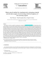
FIG. 1. Real and imaginary parts of an undamped cisoid formed
by two frequency components of equal power.
Z
fb
2(N0L)1(L/1)
Å

ͫ
z
0
z
1
иии z
L01
z
L
z
*
L
z
*
L01
иии z
*
1
z
*
0
ͬ
. (3.4)
In Fig. 1, a possible noiseless data record (real and
imaginary part of the signal) is shown. The function
It is easy to see that Z
fb
contains both Z
0fb
and

represented was generated using Eq. (2.2) with the
Z
1fb
:
parameters given in Table 1.
This function will be utilized in making a compari-
Z
fb
2(N0L)1(L/1)
Å [Z
0fb
2(N0L)1L
, c
L/1
] (3.5)
son between the Matrix Pencil Method and the Fou-
rier Transform Technique.
Z
fb
2(N0L)1(L/1)
Å [c
1
, Z
1fb
2(N0L)1L
]; (3.6)
3. TOTAL FORWARD–BACKWARD MATRIX
here c
1
and c

L/1
represent, respectively, the first and
PENCIL METHOD
(L / 1)th columns of Z
fb
.
On the other hand, the SVD of Z
fb
is
The estimation of frequencies in the presence of
Z
fb
2(N0L)1(L/1)
noise is considered by the TFBMPM. When the com-
plex exponentials in (2.2) (so-called cisoids) are un-
Å U
2(N0L)12(N0L)
S
2(N0L)1(L/1)
V
H
(L/1)1(L/1)
, (3.7)
damped
1
(which is the case in this work), to improve
the estimation accuracy we consider the matrices
Z
0fb
and Z

1fb
as defined by
TABLE 1
Input Data Considered in Fig. 1
Z
0fb
2(N0L)1L
Å
ͫ
z
0
z
1
иии z
L01
z
L01
z
*
L
z
*
L01
иии z
*
2
z
*
1
ͬ

(3.1)
64 samples (N Å 64)
Sampling period 0.25 ms (
D
t Å 1/4000 s)
2 frequency components (K Å 2)
1
Note that the Matrix Pencil Method can solve a more general
A
1
Å 1e
j2.7(p/180)
problem [1], the pole estimation, p
m
, for damped cisoids (p
m
Å
A
2
Å 1 e
j0
e
(0s
m
/jv
m
)
Dt
, s
m

§ 0, m Å 1, ,K) and the undamped cisoids are
f
1
Å 580 Hz
a particular case of the damped exponentials (in that it is enough
f
2
Å 200 Hz
to set s
m
to zero for all m).
109
6204$$0256 04-18-96 17:38:26 dspas AP: DSP
where the superscript H denotes complex conjugate and right multiplying (3.19) by Z
O
/
0fb
, the resulting
eigenproblem can be expressed astranspose of a matrix and U,
S
, and V are given by
q
H
(Z
O
1fb
Z
O
/
0fb

0
j
I)Å 0
H
, (3.20)
S
Å diag{
s
1
,
s
2
, ,
s
p
};
p Å min{2(N 0 L), L / 1} (3.8)
where Z
O
/
0fb
is the Moore–Penrose pseudoinverse [3]
of Z
ˆ
0fb
and it can be written as
s
1
§
s

2
§ rrr §
s
p
§ 0 (3.9)
U Å [u
1
, u
2
, ,u
2(N0L)
];
Z
O
/
0fb
Å (V
O
H
0
)
/
S
O
01
U
O
/
. (3.21)
Z

H
fb
u
i
Å
s
i
v
i
,iÅ 1, ,p (3.10)
Substituting (3.17) and (3.21) into (3.20), the
V Å [v
1
, v
2
, ,v
L/1
];
equivalent generalized eigen-problem becomes
Z
fb
v
i
Å
s
i
u
i
, iÅ 1, ,p (3.11)
q

H
(V
O
H
1
0
j
V
O
H
0
) Å 0
H
. (3.22)
U
H
U Å I, V
H
V Å I. (3.12)
It can be shown that (3.22) is equivalent to
s
i
are the singular values of Z
fb
and the vectors u
i
and v
i
are, respectively, the ith left singular vector
q

H
(V
O
H
1
V
O
0
0
j
V
O
H
0
V
O
0
) Å 0
H
, (3.23)
and the ith right singular vector.
The problem can be computationally improved by
which is a generalized eigenproblem of dimension K
applying the singular value filtering, which consists
1 K.
of [1] using the K largest singular values of Z
fb
, i.e.,
Using the values of the generalized eigenvalues,
j

, of (3.23), the frequency components can be esti-
Z
O
fb
2(N0L)1(L/1)
Å U
O
2(N0L)1K
S
O
K1K
V
O
H
K1(L/1)
, (3.13)
mated.
In the following, the algorithm applied to estimate
where
the frequencies is summarized as:
Step 1: Construct the matrix Z
fb
, (3.4), with the
S
O
Å diag{
s
1
,
s

2
, ,
s
K
} (3.14)
corrupted samples, where z
T
j
( j Å 0, ,L) is de-
fined as in (3.3), and L has to satisfy
has the K largest singular values of
S
and the col-
umns of U
ˆ
and V
ˆ
are formed by extracting the singu-
K £ L £ N 0 K. (3.24)
lar vectors corresponding to those K singular values.
Eq. (3.13) can be rewritten as
Step 2: Realize the SVD of Z
fb
, (3.7), and, from
its singular values, estimate K (number of frequency
Z
O
fb
Å U
O

S
O
V
O
H
Å U
O
S
O
[t
1
,t
2
, ,t
L/1
]
components). This problem is equivalent to solving
the eigenproblem Z
H
fb
Z
fb
; i.e., it can be proved that
Å [U
O
S
O
t
1
ÉU

O
S
O
t
2
rrr U
O
S
O
t
L
ÉU
O
S
O
t
L/1
]. (3.15)
the singular values of Z
fb
,
s
i
, are the nonnegative
square roots of
h
i
, where
h
i

are the eigenvalues of
Comparing (3.5), (3.6), and (3.15), the equations
the eigenproblem
Z
O
0fb
Å U
O
S
O
V
O
H
0
(3.16)
(Z
H
fb
Z
fb
0
h
i
I)r
i
Å 0. (3.25)
Z
O
1fb
Å U

O
S
O
V
O
H
1
(3.17)
Step 3: Extract V
ˆ
0
and V
ˆ
1
from V
ˆ
, (3.18), where
V
ˆ
is the K-truncation of V ((3.7) to (3.14)).
can be established, where V
ˆ
0
and V
ˆ
1
are obtained
Step 4: Estimate the K frequencies using the K
from V
ˆ

, deleting, respectively, its (L / 1)th and first
generalized eigenvalues,
j
m
, of (3.23), such that
columns, i.e.,
those eigenvalues can be expressed as
V
O
Å [V
O
0
, v
L/1
], V
O
Å [v
1
, V
O
1
]. (3.18)
j
m
Å Real(
j
m
) / j Imag(
j
m

);
By considering the matrix pencil
m Å 1, ,K, (3.26)
where Real(
j
m
) and Imag(
j
m
) are, respectively, theZ
O
1fb
0
j
Z
O
0fb
(3.19)
110
6204$$0256 04-18-96 17:38:26 dspas AP: DSP
real and imaginary parts of
j
m
, but those eigenval-
i Å 0, ,N01, (4.2.1)
ues are related to the frequencies as
has been followed, where
j
m
É e

j2p f
m
Dt
; m Å 1, ,K. (3.27)
A
m
Å ÉA
m
Ée
ju
m
; m Å 1, ,K (4.2.2)
And, from (3.26) and (3.27),
v
m
Å 2
p
f
m
; m Å 1, ,K. (4.2.3)
For the noisy data problem it is enough to consider
f
m
É
1
2
pD
t
tan
01

ͩ
Imag(
j
m
)
Real(
j
m
)
ͪ
;
(2.4), which, in vectorial notation, can be denoted
as
m Å 1, ,K. (3.28)
z Å g / w, (4.2.4)
4. LIMITS OF TFBMPM FOR FREQUENCIES
where
ESTIMATION
z
T
Å [z
0
, z
1
, ,z
N01
] (4.2.5)
4.1. The Frequency Estimation Problem
g
T

Å [g
0
, g
1
, ,g
N01
] (4.2.6)
The frequency estimation problem consists of [5,
w
T
Å [w
0
, w
1
, ,w
N01
] (4.2.7)
Chapter 6] determining the frequency components
of a signal, which obeys the mathematical model of
and those vectors could be briefly described as fol-
Section 2, from a set of noisy samples.
lows:
Any estimate of the frequency parameter evalu-
g is formed by the noise free samples, (4.2.1). This
ated from a set of samples involves a random process
vector may be seen like a deterministic unknown
and, thus, it is necessary to consider the estimate as
magnitude. The deterministic model for g is used
a random variable. Consequently, it is not correct to
when K (number of frequency components) and the

speak of a particular value of an estimate, but it is
number of snapshots (in this work just one snapshot
necessary to know its statistical distribution if the
or ‘‘picture’’ is considered) are small [9].
accuracy of the estimate is analyzed.
w represents the complex white Gaussian noise,
An efficient estimate has to be as near as possible
with the characteristics
to the true value of the parameter to be estimated
[6, Chapter 32]. This idea of ‘‘concentration’’ or ‘‘dis-
zero mean: E[w] Å 0 (4.2.8)
persion’’ about the true value may be measured us-
ing several statistical magnitudes (variance, mean
uncorrelated, with variance 2
s
2
:
squared error, etc.).
One of the first works concerned with the applica-
R
w
Å 2
s
2
I
N1N
, (4.2.9)
tion of the Estimation Theory by Fisher and Cramer
to the problem of estimating signal parameters is
where E[r] means expected value, R

w
is the correla-
that of Slepian [7]; later, in [8], the statistical the-
tion matrix of the noise, and I
N1N
is the identity
ory is applied to the estimation of the Direction of
matrix.
Arrival of a plane wave impinging on a linear phased
z is the vector containing the observed data. Ob-
array.
viously, from its definition, (4.2.4), it is a random
In this work, the limits of TFBMPM for frequency
vector.
estimation will be pointed out and the variance of
In order to define the CRB it is first necessary
this method will be compared with that of the
to introduce the joint probability density function
Cramer–Rao Bound (CRB) [6, Chapter 32].
(jpdf). The jpdf of a complex Gaussian random vec-
tor of N components, x, is defined [5, p. 478] as
4.2. The Cramer–Rao Bound
In this section, the notation
f
x
(x) Å
1
p
N
det(R

x
)
e
0 (x0E[x])
H
R
01
x
(x0E[x])
, (4.2.10)
g
i
Å
∑
K
mÅ1
ÉA
m
Ée
ju
m
e
jv
m
iDt
;
where det(r) means determinant of a matrix, H de-
111
6204$$0256 04-18-96 17:38:26 dspas AP: DSP
notes complex conjugate transpose, and 01 indicates are almost unbiased

3
in the region where the
TFBMPM works.the inverse of a matrix.
Therefore, the jpdf of w can be evaluated by using
For unbiased estimates, the CRB states that if
a
P
(4.2.8) – (4.2.10):
is an unbiased estimate of
a
, the variance of each
element,
a
P
l
(l Å 1, ,3K), of
a
P
can be no smaller
than the corresponding diagonal term in the inverse
f
w
(w) Å
1
(2
ps
2
)
N
e

01/2s
2
͚
N01
iÅ0
Éw
i
É
2
. (4.2.11)
of the Fisher Information Matrix
var(
a
P
l
) § [F
01
]
ll
, (4.2.17)
The jpdf of z can be obtained from (4.2.11) by
taking into account the relationship [10, p. 61] be-
tween z and w, which is given by (4.2.4),
where
a
P
l
is the estimate of the parameter
a
l

(l Å 1,
,3K), [F
01
]
ll
is the lth diagonal element of the
inverse of F, and F
3K13K
is the Fisher Information
f
zÉa
(zÉ
a
) Å
1
(2
ps
2
)
N
e
01/2s
2
͚
N01
iÅ0
Éz
i
0g
i

É
2
, (4.2.12)
Matrix.
The (m, n)th element of F is defined as
where É
a
denotes that the jpdf is conditioned to
an unknown vector parameter,
a
, and g
i
is given
[F]
mn
Å E
ͫ
Ì ln f
zÉa
(zÉ
a
)
Ì
a
m
r
Ì ln f
zÉa
(zÉ
a

)
Ì
a
n
ͬ
;
in (4.2.1).
From (4.2.12) one can deduce that z is a Gaussian
random vector with
m, n Å 1, ,3K. (4.2.18)
E[z] Å g (4.2.13)
The last equation, using (4.2.12), can be rewritten
[1] as
R
z
Å 2
s
2
I
N1N
. (4.2.14)
Also,
a
is the vector formed by the parameters
[F]
mn
Å
1
2
s

2
∑
N01
iÅ0
2 Real
ͫ
Ìg
i
Ì
a
m
r
Ìg*
i
Ì
a
n
ͬ
;
to be estimated. In this work the complex ampli-
tudes of the signals, A
m
,
2
and the variable
v
m
in
(4.2.1) will be chosen as unknown parameters.
m, n Å 1, ,3K, (4.2.19)

Note that A
m
is given by (4.2.2) and, therefore,
each A
m
corresponds to two parameters, ÉA
m
É and
where Real[r] denotes the real part.
u
m
. On the other hand,
v
m
is related to the frequen-
It can be proved [11] that F
01
may be decomposed
cies through (4.2.3).
as
Consequently, the vector
a
can be written as
F
01
3K13K
Å
s
2
S

3K13K
P
01
3K13K
S
3K13K
, (4.2.20)
a
T
Å [
a
1
,
a
2
,
a
3
, ,
a
3K02
,
a
3K01
,
a
3K
], (4.2.15)
where
where

S
3K13K
a
3m02
Å
v
m
Å 2
p
f
m
;
a
3m01
Å ÉA
m
É;
Å diag{[S
1
]
313
,[S
2
]
313
, ,[S
K
]
313
} (4.2.21)

a
3m
Å
u
m
; m Å 1, ,K. (4.2.16)
[S
m
]
313
Å diag{ÉA
m
É
01
,1,ÉA
m
É
01
};
The CRB provides the goodness of any estimate of
m Å 1, ,K (4.2.22)
a random parameter. The estimates of this work
have been computed via the TFBMPM, and it will
be pointed out, through simulation results, that they
P
3K13K
Å
ͫ
[P
11

]
313
иии [P
1K
]
313
Ӈ
и
и
и
Ӈ
[P
K1
]
313
иии [P
KK
]
313
ͬ
(4.2.23)
2
In order to estimate the complex amplitudes, A
m
, using the
results obtained from the TFBMPM for the frequency compo-
nents, one may solve a least-squares problem z É Ea, where z
are the corrupted samples, a contains the complex amplitudes
3
An estimate

a
P
of the vector parameter
a
is unbiased if E[
a
P
]
Å
a
.A
m
, and E is the matrix which applied to a gives g.
112
6204$$0256 04-18-96 17:38:26 dspas AP: DSP
P
mn
Å
(
D
t)
2
∑
N01
iÅ0
i
2
cos
D
(i, m, n) 0

D
t
∑
N01
iÅ0
i sin
D
(i, m, n)
D
t
∑
N01
iÅ0
i cos
D
(i, m, n)
D
t
∑
N01
iÅ0
i sin
D
(i, m, n)
∑
N01
iÅ0
cos
D
(i, m, n)

∑
N01
iÅ0
sin
D
(i, m, n)
D
t
∑
N01
iÅ0
i cos
D
(i, m, n) 0
∑
N01
iÅ0
sin
D
(i, m, n)
∑
N01
iÅ0
cos
D
(i, m, n)
(4.2.24)
r
2i
(i Å 0, ,N01), are obtained to construct the

D
(i, m, n) Å i(
v
m
0
v
n
)
D
t /
u
m
0
u
n
;
complex sequence
i Å 0, ,N01; m, n Å 1, ,K. (4.2.25)
x
i
Å r
1i
/ jr
2i
; i Å 0, ,N01. (4.3.1.1)
4.3. Simulation Results
4.3.1. Input Data. In this section several graphs
Taking into account that the variance of the com-
are presented and discussed in order to facilitate a
plex noise, w

i
, was defined as 2
s
2
, it is easy to de-
better understanding of the TFBMPM and its esti-
duce the relationship
mation limits.
The methodology followed to obtain the different
plots has been to generate a set of N complex sam-
w
i
Å

2
s
2
x
i
; i Å 0, ,N01. (4.3.1.2)
ples, using ((4.2.1) to (4.2.4)) and then to apply the
TFBMPM as proposed in the algorithm of Section 3.
The SNR, for each frequency component, has been
This algorithm was iterated several times when the
defined as
variance of the frequency estimate was numerically
computed.
The input data may be described as follows:
SNR
m

Å 10 log
10
ÉA
m
É
2
2
s
2
;
(1) Observation interval
8 samples have been considered (N Å 8).
m Å 1, ,K. (4.3.1.3)
The sampling period was normalized
(
D
t Å 1 s).
(4) TFBMPM remarks (see Section 3)
(2) Description of the signal
The first step in the TFBMPM consists of choosing
2 frequency components have been chosen
a value for the pencil parameter, L, in order to form
(K Å 2).
the Z
fb
matrix.
ÉA
1
É Å ÉA
2

É Å 1: Two components of equal
The best choice for L is [2]
power.
u
1
,
u
2
: A deterministic model has been as-
sumed for the phases of the frequency components.
N
3
£ L £
2N
3
, (4.3.1.4)
The difference
u
1
0
u
2
is taken from values in [0Њ,
180Њ ). TFBMPM performance depending on
u
1
0
u
2
is shown in the next section.

but, at the same time, L has to satisfy (3.24).
f
1
Å 0.200 Hz.
To numerically compute the variance of the fre-
f
2
: The second frequency varies between
quencies the algorithm proposed in Section 3 has
0.270 and 0.290 Hz and, therefore, the value of
D
f
been iterated 500 times (trials). For each trial, a
studied is in the interval [0.070 Hz, 0.090 Hz],
different vector w was randomly taken.
where
D
f Å f
2
0 f
1
.
(3) Statistical considerations for the noise (see 4.3.2. Performance of the TFBMPM as a function
of
u
1
0
u
2
. The accuracy in the frequencies estima-Section 4.2)

The noise was generated by using ISML [12] FOR- tion, using the TFBMPM, depends strongly on the
difference of phases between the components of theTRAN subroutine GGNML. This subroutine is a
Gaussian (0, 1) pseudo-random number generator. signal. It has been proved [2] that the inverse of the
variance of the frequencies estimates,With GGNML two sets of N real numbers, r
1i
and
113
6204$$0256 04-18-96 17:38:26 dspas AP: DSP
FIG. 2. Inverse of the variance of the first frequency estimate, as a function of the difference of phases of the two frequency components
and the difference of frequencies. SNR Å 17 dB and the pencil parameter for the TFBMPM is L Å 5.
have been explained in Section 4.3.1. SNR is 17 dB
10 log
10
1
var(f
O
m
)
; m Å 1, ,K, (4.3.2.1)
and L Å 5. In Fig. 3 the same input data are taken,
and the CRB for the variance of f
ˆ
1
is shown. To
obtain this 3D plot, the method in Section 4.2 has
reaches a maximum if
been followed, determining the CRB for the variance
of
v
P

1
and applying the relationship in (4.2.3) to cal-
(
v
m
0
v
n
)(N 0 1)
D
t / 2(
u
m
0
u
n
)
culate the CRB for f
ˆ
1
.
Å (2l)
p
(4.3.2.2)
Comparing Fig. 2 to Fig. 3 one can deduce that
the CRB is reached by the estimate obtained using
and a minimum if
TFBMPM when f
2
0 f

1
is close to 0.090 Hz or, in the
entire interval [0.070 Hz, 0.090 Hz], when
u
1
0
u
2
(
v
m
0
v
n
)(N 0 1)
D
t / 2(
u
m
0
u
n
)
is far from the worst case.
4.3.3. Estimating the number of frequency compo-
Å l
p
. (4.3.2.3)
nents from the singular values of Z
fb

. As was ex-
plained in Section 3, to estimate the number of fre-
In both Eqs. (4.3.2.2) and (4.3.2.3), m, n, and l
quency components K the eigenvalues of Z
H
fb
Z
fb
will
have to satisfy
be used. This idea will be followed in this section for
both the ideal sampling (neglecting the noise) and
for all m x n; m, n Å 1, ,K;
the corrupted samples.
l integer. (4.3.2.4)
Figures 4 to 11 show the normalized magnitude,
in dB, of the eigenvalues,
j
n
(n Å 1, ,L/1), of
We will call, respectively, best case and worst case
Z
H
fb
Z
fb
. This normalized magnitude is given by
to (4.3.2.2) and (4.3.2.3). The meaning is simple; when
(4.3.2.2) is given, (4.3.2.1) reaches a maximum and
thus the variance takes its minimum value. In other

10 log
10
j
n
j
max
; n Å 1, ,L/1, (4.3.3.1)
words, the distribution of the estimates reaches its
maximum of concentration around the true value of
the vector parameter being estimated. The explana-
tion for the worst case is analogous. where L is the pencil parameter and
j
max
is the
largest eigenvalue.In Fig. 2 that dependence is shown. The input data
114
6204$$0256 04-18-96 17:38:26 dspas AP: DSP
FIG. 3. Inverse of the CRB of the first frequency estimate, as a function of the difference of phases of the two frequency components
and the difference of frequencies. SNR Å 17 dB.
The input data for SNR, L, f
2
0 f
1
, and
u
1
0
u
2
are number of signals is estimated from the K largest

eigenvalues of Z
H
fb
Z
fb
). This gap is much greater forgiven in Table 2.
Comparing the noiseless case (Figs. 4 to 7) to the the noiseless samples than for the samples in noise,
as was expected. In fact, the noise is the ‘‘culprit’’ ofcorrupted samples (Figs. 8 to 11) one can see that
the main difference is the ‘‘gap’’ between the second the gap reduction.
To enhance this gap, for the noisy data case, digi-eigenvalue and the third one (note that two fre-
quency components are being considered and the tal filtering techniques in the original set of samples,
z
i
, can be applied [13].
FIG. 5. Normalized magnitude of the eigenvalues of Z
H
fb
Z
fb
. TheFIG. 4. Normalized magnitude of the eigenvalues of Z
H
fb
Z
fb
. In-
put data: N Å 8, K Å 2, É A
1
É Å ÉA
2
É Å 1,

u
1
0
u
2
Å 88.2Њ (worst same input data as in Fig. 4, but
u
1
0
u
2
Å 113.4Њ (worst case)
and f
2
Å 0.290 Hz.case), f
2
Å 0.270 Hz, f
1
Å 0.200 Hz, SNR Å ϱ (noiseless), L Å 3.
115
6204$$0256 04-18-96 17:38:26 dspas AP: DSP
FIG. 6. Normalized magnitude of the eigenvalues of Z
H
fb
Z
fb
. The
FIG. 8. Normalized magnitude of the eigenvalues of Z
H
fb

Z
fb
. The
same input data as in Fig. 4, but
u
1
0
u
2
Å 178.2Њ (best case) and
same input data as in Fig. 4, but SNR Å 20 dB.
L Å 6.
ance of f
ˆ
1
is referred to the CRB, which means that
4.3.4. TFBMPM for frequencies estimation in
the (SNR) – ( f
2
0 f
1
) plane represents the CRB. Both
presence of noise. In this section the number of fre-
figures demonstrate that the TFBMPM works be-
quency components, K, is assumed to be known and
yond a certain threshold of SNR.
equal to 2.
Consequently, the threshold is an indicator of the
Figures 12 and 13 show the TFBMPM perfor-
estimation limits. For example, for the worst case,

mance as a function of SNR and f
2
0 f
1
. Figure 12
and for f
2
0 f
1
Å 0.070 Hz, the threshold is between
has been obtained for the worst case of
u
1
0
u
2
ac-
17 and 19 dB, as is shown in Fig. 12; therefore this
cording to (4.3.2.3), while Fig. 13 corresponds to the
is the SNR lower limit in order for the TFBMPM to
best case estimation, (4.3.2.2). Note that the vari-
provide reasonable results.
FIG. 7. Normalized magnitude of the eigenvalues of Z
H
fb
Z
fb
. The
same input data as in Fig. 4, but
u

1
0
u
2
Å 23.4Њ (best case), f
2
FIG. 9. Normalized magnitude of the eigenvalues of Z
H
fb
Z
fb
. The
same input data as in Fig. 5, but SNR Å 20 dB.Å 0.290 Hz, and L Å 6.
116
6204$$0256 04-18-96 17:38:26 dspas AP: DSP
TABLE 2
Input Data Considered for Figs. 4 to 11
Figure SNR (dB) Lf
2
–f
1
(Hz)
u
1
–
u
2
(Њ)
4 ϱ (noiseless) 3 0.070 88.2 (worst case)
5 ϱ (noiseless) 3 0.090 113.4 (worst case)

6 ϱ (noiseless) 6 0.070 178.2 (best case)
7 ϱ (noiseless) 6 0.090 23.4 (best case)
8 20 3 0.070 88.2 (worst case)
9 20 3 0.090 113.4 (worst case)
10 20 6 0.070 178.2 (best case)
11 20 6 0.090 23.4 (best case)
For the best estimate, and f
2
0 f
1
Å 0.070 Hz, the
5. THE FOURIER TRANSFORM ESTIMATOR
lower limit is between 5 and 6 dB, as is shown in
Fig. 13.
Figures 14 and 15 have been extracted from the
5.1. The Periodogram
data used in Figs. 2 and 3 and thus correspond to a
The Fourier Transform Estimator (FTE) for fre-
SNR of 17 dB. Also 0.070 Hz is the designated value
quency components estimation considered in this
for f
2
0 f
1
in Fig. 14 and 0.090 Hz is the value in
work is based on the classic periodogram. The esti-
Fig. 15.
mates of the frequencies, f
ˆ
m

(m Å 1, , K), will
In Fig. 14 the CRB is reached for all
u
1
0
u
2
be the values of the variable f (frequency) which
except in the interval (70Њ, 105Њ ), approximately,
maximize (local maxima) the periodogram, ( f ).
where the TFBMPM is not performing well. The
The periodogram is an estimate of the power density
reason can be found in Fig. 12, obtained for the
spectrum and can be defined [14] as
worst case of
u
1
0
u
2
, where one can see that for f
2
0 f
1
Å 0.070 Hz, a SNR of 17 dB is below the thresh-
( f ) Å
1
N
D
t

ÉZ( f )É
2
, (5.1.1)
old and, by definition, the estimator ceases func-
tioning. Nevertheless, the CRB is always reached
in Fig. 15 because 17 dB is above the threshold
for all
u
1
0
u
2
(for the worst case estimation the
where Z( f ) is the Discrete-Time Fourier Transform
threshold for f
2
0 f
1
Å 0.090 Hz is between 13 and
(DTFT) of the noise samples,
14 dB, as is shown in Fig. 12).
FIG. 10. Normalized magnitude of the eigenvalues of Z
H
fb
Z
fb
. FIG. 11. Normalized magnitude of the eigenvalues of Z
H
fb
Z

fb
.
The same input data as in Fig. 7, but SNR Å 20 dB.The same input data as in Fig. 6, but SNR Å 20 dB.
117
6204$$0256 04-18-96 17:38:26 dspas AP: DSP
FIG. 12. Variance of f
O
1
compared to the CRB for the worst case estimation. The peaks show the threshold of the TFBMPM.
z(i
D
t) Å z
original
(i
D
t)rh(i
D
t),
Z( f ) Å
D
t
∑
N01
iÅ0
z
i
e
0j2pfiDt
, 0
1

2
D
t
£ f £
1
2
D
t
.
i Å 0,1, ,N01 (5.2.2)
(5.1.2)
h(i
D
t) Å
ͭ
1, 0 £ i
D
t £ (N 0 1)
D
t
0, otherwise.
(5.2.3)
Figure 16 shows the normalized periodogram for
the complex signal of Fig. 1. Note that the SNR as-
sumed for this example is ϱ (noiseless samples).
In terms of the DTFT the finite record is periodi-
The two main peaks correspond to the two frequency
cally extended, in the time domain, with period
components of the signal.
N

D
t. If this period does not match the natural
period of the signal, discontinuities appear at the
5.2. Consequences of the Leakage Effect for
boundaries of the record. These discontinuities
Frequencies Estimation
[16] are the cause of the leakage. The function of
It is well known [15, pp. 136–144] that side lobes
a window is to reduce them. For this reason it is
(see Fig. 16) appear in the DTFT of a finite length
required that a window go to zero smoothly at its
sequence, z
i
(i Å 0, ,N01). This phenomenon,
boundaries.
called leakage, becomes more evident when the fre-
Even if an appropriate window can reduce the
quencies move closer or when one frequency compo-
bias of the frequency estimate, the application of
nent is much stronger than the rest.
a window has a disadvantage as it decreases the
In order to mitigate the leakage effect, windows
spectral resolution. Consequently, one has to
(weighting functions) are used. An observation in-
make a trade-off between the spectral resolution
terval, N
D
t, is equivalent to a rectangular window,
desired and the reduction of the side lobes. In any
h(i

D
t), applied to the original signal, resulting in a
case, the spectral resolution, in Hz, is limited [15,
finite set of samples, z(i
D
t):
pp. 46–49] to the reciprocal of the observation
time, (N
D
t)
01
. Therefore, frequency components
separated by a distance less than (N
D
t)
01
will not
z
original
(i
D
t) defined for
be distinguished by the FTE, that is, the case of
simulations carried out in Section 4.3, wherei Å0ϱ, ,01,0,1, ,/ϱ (5.2.1)
118
6204$$0256 04-18-96 17:38:26 dspas AP: DSP
FIG. 13. Variance of f
O
1
compared to the CRB for the best case estimation. The peaks show the threshold of the TFBMPM.

(N
D
t)
01
is 0.125 Hz and the maximum
D
f studied In Figs. 17 and 18 the windows are shown in both
time and frequency domains. The number of samplesis 0.090 Hz and, in consequence, the FTE does not
work under those conditions. has been taken as 12 and the sampling period is 0.25
ms. The main difference among these windows is theThree windows have been considered in this work:
Rectangular window reduction in the side lobes. The Standard window
achieves the largest reduction of the bias, but it does
so at the expense of broadening the main lobe, which
h
i
Å
ͭ
1, 0 £ i £ N 0 1
0, otherwise;
(5.2.4)
results in a loss of spectral resolution.
The window in the time domain is applied by
weighting the input samples, z
i
, with the window
Standard window [11]
coefficients, h
i
, by modifying Eq. (5.1.2) in the fol-
lowing way:

h
i
Å
1
3
∑
3
kÅ0
a
k
cos
ͩ
2
p
ik
N
ͪ
,0£i£N01
0, otherwise;
Z( f ) Å
D
t
∑
N01
iÅ0
z
i
h
i
e

0j2pfiDt
, 0
1
2
D
t
£ f £
1
2
D
t
.
(5.2.5)
(5.2.7)
with a
0
Å 1, a
1
Å01.43596, a
2
Å 0.497536, a
3
Å
Eq. (5.2.7) is simply the DTFT of the weighted
00.061576.
samples, z
i
h
i
, and it will be used, jointly with

Kaiser window [17, p. 232]
(5.1.1), to estimate the frequency components.
5.3. Comparison between the FTE and the
h
i
Å
I
0
[
b
r

1 0 ((i 0 N/2)/N/2)
2
]
I
0
[
b
]
,
TFBMPM
0 £ i £ N 0 1
The frequency component estimation using the
0, otherwise;
Fourier Transform has been widely studied by
Rife and Boorstyn in [11]. Figure 19 provides the
(5.2.6)
comparison between various windows and the
TFBMPM.here I

0
[r] is the modified Bessel function of the first
kind and order zero and
b
is a parameter, and in The input data for Fig. 19 are given by Fig. 1,
and the SNR, which is defined in (4.3.1.3), variesthis work it has been chosen according to Table 3.
119
6204$$0256 04-18-96 17:38:26 dspas AP: DSP
reduction of the bias but at the expense of increasing
the variance of the estimate.
The bias shown in Fig. 20 was computed according
to
bias(f
O
1
) Å E[f
O
1
] 0 f
1
, (5.3.3)
and one can see that for SNR below 10 dB the FTE
with the Standard window offers less bias than the
TFBMPM. Nevertheless, the rmse obtained with the
TFBMPM is less than the one computed using the
Standard window as seen in Fig. 19. This is because
the Standard window reduces the bias but at the
same time increases the variance. On the other
hand, the use of the Rectangular window makes a
FTE biased even for high SNR.

In Fig. 21 the behavior of the estimator as the
number of samples increases is shown. The input
data are the same as in Fig. 19, but a
Du
of worst
case was taken for each N, and SNR Å 0 dB. The
FTE uses the Kaiser window for this simulation and
FIG. 14. Comparison between the inverse of the variance and
it can be seen that for long data record the FTE
the CRB for the first frequency estimate. f
2
0 f
1
Å 0.070 Hz and
reaches the CRB.
SNR Å 17 dB. The TFBMPM produces inaccurate results in
u
1
0
u
2
√ (70Њ, 105Њ ) because the SNR is below the threshold.
Figure 22 shows a comparative study of the rmse
as a function of the difference of frequencies f
1
0 f
2
for two components of equal power when the SNR is
between 0 and 40 dB. The values corresponding to
20 dB. As in Fig. 19 the sampling period is 0.25

the CRB (dark squares in Fig. 19) have been com-
ms but the number of samples has been drastically
puted by the square root of the corresponding diago-
nal term in the inverse of the Fisher Information
Matrix (4.2.20) and the pencil parameter, L, for the
TFBMPM has been taken as 22. The statistical mag-
nitude represented in Fig. 19 is the root mean
squared error (rmse), defined as
rmse(f
O
1
) Å

E[(f
O
1
0 f
1
)
2
] , (5.3.1)
where E[r] means expected value, f
ˆ
1
is the parame-
ter being estimated, and f
1
is the true value of the
parameter. The rmse is related to the variance
through the bias, i.e.,

rmse
2
(f
O
1
) Å bias
2
(f
O
1
) / var(f
O
1
), (5.3.2)
and, evidently, for unbiased estimators the rmse be-
comes the square root of the variance. The rmse was
computed using 200 trials for each algorithm.
From Fig. 19 one can see that the TFBMPM is
performing better than the FTE in all the SNR
range. On the other hand, and in spite of the smaller
bias presented by the Standard window (see Fig.
FIG. 15. Comparison between the inverse of the variance and
20), the Kaiser window provides better results than
the CRB for the first DOA estimate. f
2
0 f
1
Å 0.090 Hz and SNR
the Standard window for SNR below 30 dB. The rea-
Å 17 dB. The TFBMPM reaches the CRB for all

u
1
0
u
2
because
the SNR is above the threshold.
son for this is that the Standard window achieves a
120
6204$$0256 04-18-96 17:38:26 dspas AP: DSP
FIG. 16. Normalized periodogram of the undamped cisoid of Fig. 1. A Rectangular window was used to weight the samples in the time
domain.
reduced from 64 to 12 samples. The pencil parameter The last simulation included in this paper is
shown in Figs. 24 to 28. While in the previous simu-for the TFBMPM is L Å 7, f
2
is 200 Hz, and
Du
(worst case) is assumed according to (5.3.2.3). Two lations the two frequency components had the same
power, in Figs. 24 to 28, the first frequency compo-main conclusions can be drawn from Fig. 22; on the
one hand the FTE does not work for
D
f below 460 nent has 10 times more power than the second one,
Hz ((N
D
t)
01
is 333 Hz) while TFBMPM still per-
forms well up to 180 Hz and, on the other hand, the
TFBMPM performs better than the FTE even when
FTE works, i.e., for

D
f greater than 460 Hz.
In Fig. 23 the accuracy of the estimators de-
pending on the number of samples, N, is shown. A
SNR of 15 dB for two frequency components of equal
power at, respectively, 1300 and 1000 Hz was consid-
ered. Also a
D
t of 0.25 ms and a
Du
of worst case
for each N were taken. Similar conclusions to the
ones for Fig. 22 can be derived.
TABLE 3
b
Values for the Kaiser Window
Figure
b
Value
17, 18, 19, 20, 21, 22 6
FIG. 17. The three windows used in this work for the Fourier
23 5.5
Transform Estimator (FTE). The graph shows 12 samples for
24, 25, 26, 27 5
each of them in the time domain.
121
6204$$0256 04-18-96 17:38:26 dspas AP: DSP
FIG. 20. Bias for the estimate of Fig. 19. In spite of the fact
FIG. 18. Comparative spectrum of the windows. The Discrete
that the Standard window offers less bias than the TFBMPM for

Time Fourier Transform (DTFT) was used to obtain H( f ).
SNR below 10 dB, its rmse performance is worse because the
Standard window increases the variance.
i.e., É A
1
É
2
Å 10 ÉA
2
É
2
, which supposes that SNR
1
ter used in the TFBMPM is 6, f
2
Å 400 Hz, SNR
2
Å
(dB) Å 10 dB / SNR
2
(dB). On the other hand, 0.25
10 dB, and
Du
of worst case for each
D
f is chosen.
ms for the sampling period and 12 samples charac-
From Figs. 24 and 25 one can see the better perfor-
terize the observation interval. The pencil parame-
mance of the TFBMPM for both f

ˆ
1
and f
ˆ
2
estimates
and also a larger spectral resolution for this estima-
tor. At this point it is important to indicate that the
FIG. 19. A first comparison between the TFBMPM and the FTE.
Several SNR were considered for the signal of Fig. 1. A better
performance of the TFBMPM is observed in the entire SNR range FIG. 21. The signal of Fig. 1 was contaminated with a SNR Å
0 dB. For long data records the FTE reaches the CRB.under study.
122
6204$$0256 04-18-96 17:38:26 dspas AP: DSP
FIG. 22. The signal was built with two components of equal
FIG. 24. rmse of the first estimate, f
O
1
, for a signal composed by
power and SNR Å 20 dB. The observation interval is character-
two frequency components. The first component has 10 times
ized by 12 samples and
D
t Å 0.25 ms. Better performance and
more power than the second one. SNR
2
Å 10 dB.
higher spectral resolution are observed for the TFBMPM.
27, where the main lobe, centered in 1000 Hz ( f
1

),
criterion applied to consider whether an estimate is
is masking the lobe corresponding to the second fre-
valid, when the FTE is used, has consisted of being
quency component, f
2
, at 400 Hz. The Rectangular
able to distinguish the two frequency components.
window was not considered in this simulation be-
This idea is reflected in Fig. 26, where the Kaiser
cause, for some frequencies, the smaller frequency
window is used for the FTE, f
1
is 1400 Hz, f
2
is 400
component, f
2
, was hidden for side lobes, as is shown
Hz, and
Du
Å 45Њ. The opposite case is shown in Fig.
in Fig. 28. The two frequency components of the sig-
nal for that example are f
1
Å 1860 Hz and f
2
Å 400
Hz, and
Du

Å 177.3Њ.
FIG. 23. A dual behavior to the one of Fig. 21 is derived. A SNR
of 15 dB was chosen for two components of equal power and 300 FIG. 25. The same input data as in Fig. 23 but the estimate
evaluated is f
O
2
.Hz apart.
123
6204$$0256 04-18-96 17:38:26 dspas AP: DSP
FIG. 28. For some difference of frequencies, the second main
FIG. 26. The two main lobes centered, respectively, at 1400 and
lobe is hidden by side lobes when the Rectangular window is
400 Hz, can be distinguished from each other. The first main lobe
applied and, consequently, the FTE will not work.
has 10 times more power than the second one.
6. CONCLUSIONS
the expense of spectral resolution. The Rectangular,
Standard, and Kaiser windows have been chosen as
the representatives for numerical simulation. It has
The objective of this paper has been to present the
been shown that when TFBMPM works beyond a
TFBMPM and the Fourier Transform Technique for
certain threshold of SNR, it provides better variance
the estimation of undamped cisoids in white
estimates than the Fourier techniques, although the
Gaussian noise. The accuracy of TFBMPM has been
bias may be large. However, the root mean squared
brought out in the presence of noise and its variance
error is less for the TFBMPM than for the Fourier
compared to that of the Cramer–Rao Bound.

Techniques with various windows.
It has been shown that applying windowing in the
Fourier Transform provides unbiased estimates at
REFERENCES
1. Hua, Y., and Sarkar, T. K. Matrix pencil method for estimat-
ing parameters of exponentially damped/undamped sinu-
soids in noise. IEEE Trans. Acoust. Speech Signal Process.
38, No. 5 (May 1990), 814–824.
2. Hua, Y. On techniques for estimating parameters of exponen-
tially damped/undamped sinusoids in noise. Ph.D. disserta-
tion, Syracuse University, New York, Aug. 1988.
3. Golub, G. H., and Van Loan, C. F. Matrix Computations. The
John Hopkins Univ. Press, Baltimore, 1985.
4. Hua, Y., and Sarkar, T. K. Matrix pencil method and its
performance. In Proc. ICASSP-88, New York, 1988, pp. 2476–
2479.
5. Johnson, D. H., and Dudgeon, D. E. Array Signal Processing:
Concepts and Techniques. Prentice Hall, Englewood Cliffs,
NJ, 1994.
6. Cramer, H. Mathematical Methods of Statistics. Princeton
Univ. Press, Princeton, NJ, 1966.
7. Slepian, D. Estimation of signal parameters in the presence
of noise. IRE Trans. Inform. Theory PGIT-3 (March 1954),
68–89.
FIG. 27. The first main lobe, at 1000 Hz, is masking the second 8. Brennan, L. E. Angular accuracy of phased array radar. IRE
Trans. Antennas Propagation AP-9 (May 1961), 268–275.main lobe centered at 400 Hz.
124
6204$$0256 04-18-96 17:38:26 dspas AP: DSP
9. Hua, Y., and Sarkar, T. K. A. Note on the Cramer–Rao bound NY. He came to Syracuse with a fellowship from the Marcelino
Botı

B
n Foundation (Santander, Spain). He is currently workingfor 2-d direction finding based on 2-d array. IEEE Trans.
Signal Process. 39, No. 5 (May 1991), 1215–1218. toward his Ph.D. degree in the University of Cantabria, studying
different topics related to applied electromagnetics. His research
10. Shanmugan, K. S., and Breipohl, A. M. Random Signals:
interests include signal processing and electromagnetic compati-
Detection, Estimation and Data Analysis. Wiley, New York,
bility.
1988.
TAPAN KUMAR SARKAR was born in Calcutta, India, on Au-
11. Rife, D. C., and Boorstyn, R. R. Multiple tone parameter esti-
gust 2, 1948. He received the B. Tech. degree from the Indian
mation from discrete-time observations. Bell System Tech. J.
Institute of Technology, Kharagpur, India, in 1969, the M.Sc.E.
55, No. 9 (Nov. 1976), 1389–1410.
degree from the University of New Brunswick, Fredericton, Can-
12. IMSL, INC. IMSL Library. Problem-Solving Software Sys-
ada, in 1971, and the M.S. and Ph.D. degrees from Syracuse Uni-
tems for Mathematical and Statistical FORTRAN Program-
versity, Syracuse, NY in 1975. From 1975 to 1976 he was with
ming. Nov. 1984.
the TACO Division of the General Instruments Corporation. He
13. Sarkar, T. K., Hu, F., Hua, Y., and Wicks, M. A real-time
was with the Rochester Institute of Technology, Rochester, NY,
signal processing technique for approximating a function by
from 1976 to 1985. He was a Research Fellow at the Gordon
a sum of complex exponentials utilizing the matrix-pencil
McKay Laboratory, Harvard University, Cambridge, MA, from
approach. Digital Signal Process. 4, (1994), 127–140.
1977 to 1978. He founded OHRN Enterprises in 1985, which has

14. Kay, S. M., and Marple, S. L., Jr. Spectrum analysis—A mod-
been engaged in signal processing research and development,
ern perspective. Proc. IEEE 69, No. 11 (Nov. 1981), 1380–
with several governmental and industrial organizations. He is
1419.
also a professor in the Department of Electrical and Computer
Engineering, Syracuse University, Syracuse, NY. His current re-
15. Marple, S. L., Jr. Digital Spectral Analysis with Applications.
search interests deal with adaptive polarization processing and
Prentice Hall, Englewood Cliffs, NJ, 1987.
numerical solutions of operator equations arising in electromag-
16. Harris, F. J. On the use of windows for harmonic analysis
netics and signal processing with application to radar system
with the discrete Fourier transform. Proc. IEEE 66, No. 1
design. He obtained one of the ‘‘best solution’’ awards in May
(Jan 1978), 51–83.
1977 at the Rome Air Development Center (RADC) Spectral Esti-
17. Kuo, F. F., and Kaiser, J. F. System Analysis by Digital Com-
mation Workshop. He has authored or coauthored more than 154
puter. Wiley, New York, 1966.
journal articles and conference papers and has written chapters
in eight books. Dr. Sarkar is a registered professional engineer
in the State of New York. He received the Best Paper Award of
the IEEE Transactions on Electromagnetic Compatibility in 1979.
He was an Associate Editor for feature articles of the IEEE Anten-
JOSE ENRIQUE FERNANDEZ DEL RIO was born in Santon
˜
a,
nas and Propagation Society Newsletter, the Technical Program
Cantabria, Spain, on December 28, 1965. He graduated in 1992

Chairman for the 1988 IEEE Antennas and Propagation Society
as the valedictorian of his class with a B.S. degree in Physics–
International Symposium and URSI Radio Science Meeting, and
Electronics from the University of Cantabria, Santander, Spain.
an Associate Editor of the IEEE Transactions of Electromagnetic
In 1994 he received the M.S. degree in Electrical Engineering,
Compatibility. He was an Associate Editor of the Journal of Elec-
also from the University of Cantabria. For two years he was a
tromagnetic Waves and Applications and on the editorial board
member of a research team of the University of Cantabria, where
of the International Journal of Microwave and Millimeter Wave
he worked on POWERCAD, a project which is part of ESPRIT,
Computer Aided Engineering. He has been appointed U.S. Re-
one of the research programs sponsored by the European Commu-
search Council Representative to many URSI General Assem-
nity. His task consisted in modeling the inductive coupling and
blies. He is the Chairman of the Intercommission Working Group
the radiated noise in switched mode power Supplies. From 1994
of International URSI on Time Domain Metrology. Dr. Sarkar is
to 1995 he was a visiting scholar in the Department of Electrical
a member of Sigma Xi and International Union of Radio Science
Commissions A and B.and Computer Engineering at Syracuse University, Syracuse,
125
6204$$0256 04-18-96 17:38:26 dspas AP: DSP