The yield gap of global grain production-A spatial analysis
Bạn đang xem bản rút gọn của tài liệu. Xem và tải ngay bản đầy đủ của tài liệu tại đây (840.74 KB, 11 trang )
The yield gap of global grain production: A spatial analysis
Kathleen Neumann
a,
*
, Peter H. Verburg
b
, Elke Stehfest
c
, Christoph Müller
c,d
a
Land Dynamics Group, Wageningen University, P.O. Box 47, 6700 AA Wageningen, The Netherlands
b
Institute for Environmental Studies, VU University Amsterdam, De Boelelaan 1087, 1081 HV Amsterdam, The Netherlands
c
Netherlands Environmental Assessment Agency (PBL), P.O. Box 303, 3720 AH Bilthoven, The Netherlands
d
Potsdam Institute for Climate Impact Research (PIK), Telegrafenberg, P.O. Box 601203, 14412 Potsdam, Germany
article info
Article history:
Received 14 April 2009
Received in revised form 29 January 2010
Accepted 22 February 2010
Available online 26 March 2010
Keywords:
Grain production
Yield gap
Land management
Intensification
Inefficiency
Frontier analysis
abstract
Global grain production has increased dramatically during the past 50 years, mainly as a consequence of
intensified land management and introduction of new technologies. For the future, a strong increase in
grain demand is expected, which may be fulfilled by further agricultural intensification rather than
expansion of agricultural area. Little is known, however, about the global potential for intensification
and its constraints. In the presented study, we analyze to what extent the available spatially explicit glo-
bal biophysical and land management-related data are able to explain the yield gap of global grain pro-
duction. We combined an econometric approach with spatial analysis to explore the maximum attainable
yield, yield gap, and efficiencies of wheat, maize, and rice production. Results show that the actual grain
yield in some regions is already approximating its maximum possible yields while other regions show
large yield gaps and therefore tentative larger potential for intensification. Differences in grain produc-
tion efficiencies are significantly correlated with irrigation, accessibility, market influence, agricultural
labor, and slope. Results of regional analysis show, however, that the individual contribution of these fac-
tors to explaining production efficiencies strongly varies between world-regions.
Ó 2010 Elsevier Ltd. All rights reserved.
1. Introduction
Human diets strongly rely on wheat (Triticum aestivum L.), maize
(Zea mays L.), and rice (Oryza sativa L.). Their production has in-
creased dramatically during the past 50 years, partly due to area
extension and new varieties but mainly as a consequence of inten-
sified land management and introduction of new technologies
(Cassman, 1999; Wood et al., 2000; FAO, 2002a; Foley et al.,
2005). For the future, a continuous strong increase in the demand
for agricultural products is expected (Rosegrant and Cline, 2003).
It is highly unlikely that this increasing demand will be satisfied
by area expansion because productive land is scarce and also
increasingly demanded by non-agricultural uses (Rosegrant et al.,
2001; DeFries et al., 2004). The role of agricultural intensification
as key to increasing actual crop yields and food supply has been dis-
cussed in several studies (Ruttan, 2002; Tilman et al., 2002; Barbier,
2003; Keys and McConnell, 2005). However, in many regions,
increases in grain yields have been declining (Cassman, 1999;
Rosegrant and Cline, 2003; Trostle, 2008). Inefficient management
of agricultural land may cause deviations of actual from potential
crop yields: the yield gap. At the global scale little information is
available on the spatial distribution of agricultural yield gaps and
the potential for agricultural intensification. There are three main
reasons for this lack of information.
First of all, little consistent information of the drivers of agricul-
tural intensification is available at the global scale. Keys and
McConnell (2005) have analyzed 91 published studies of intensifi-
cation of agriculture in the tropics to identify factors important for
agricultural intensification. They emphasize that a plentitude of
factors drive changes in agricultural systems. The relative contri-
bution of them varies greatly between regions. This problem was
confirmed by a number of studies that have investigated grain
yields, and tried to identify factors that either support or hamper
grain production at different scales (Kaufmann and Snell, 1997;
Timsina and Connor, 2001; FAO, 2002a; Reidsma et al., 2007).
These studies also indicate that most of these factors are locally
or regionally specific, which makes it difficult to derive a general-
ized set of factors that apply to all countries. A second reason for
the absence of reliable information on the global yield gap is the
limited availability of consistent data at the global scale. Especially
land management data are lacking. When it comes to quantifying
potential changes in crop yields often only biophysical factors,
such as climate are considered while constraints for increasing ac-
tual crop yields are often neglected or captured by a simple man-
agement factor that is supposed to include all factors that cause
0308-521X/$ - see front matter Ó 2010 Elsevier Ltd. All rights reserved.
doi:10.1016/j.agsy.2010.02.004
* Corresponding author. Tel.: +31 317 482430; fax: +31 317 419000.
E-mail addresses: (K. Neumann), Peter.Verburg@
ivm.vu.nl (P.H. Verburg), (E. Stehfest), christoph.mueller@
pik-potsdam.de (C. Müller).
Agricultural Systems 103 (2010) 316–326
Contents lists available at ScienceDirect
Agricultural Systems
journal homepage: www.elsevier.com/locate/agsy
a deviation from potential yields (Alcamo et al., 1998; Harris and
Kennedy, 1999; Ewert et al., 2005; Long et al., 2006). Finally, lack
of data also leads to another difficulty. Many yield gap analyses
have in common that they apply crop models for simulating poten-
tial crop yields which are compared to actual yields (Casanova
et al., 1999; Rockstroem and Falkenmark, 2000; van Ittersum
et al., 2003). Potential yields, however, are a concept describing
crop yields in absence of any limitations. This concept requires
assumptions on crop varieties and cropping periods. While such
information is easily attainable at the field scale it is not available
at the global scale. Moreover, different simplifications of crop
growth processes exist between the models. This may result in
uncertainties of globally simulated potential yields, and makes an
appropriate model calibration essential for global applications.
Comparing simulated global crop yields to actual yields therefore
bears the risk of dealing with error ranges and uncertainties of dif-
ferent data sources (i.e., observations and simulation results)
which might even outrange the yield gap itself.
Consequently, available knowledge about the yield gap is rather
inconsistent and regional and global levels of agricultural produc-
tion have hardly been studied together.
The aim of this paper is to overcome some of the mentioned
shortcomings by analyzing actual yields of wheat, maize, and rice
production at both regional and global scale accounting for bio-
physical and land management-related factors. We propose a
methodology to explain the spatial variation of the potential for
intensification and identifying the nature of the constraints for fur-
ther intensification. We estimated a stochastic frontier production
function to calculate global datasets of maximum attainable grain
yields, yield gaps, and efficiencies of grain production at a spatial
resolution of 5 arc min (approximately 9.2 Â 9.2 km on the equa-
tor). Applying a stochastic frontier production function facilitates
estimating the yield gap based on the actual grain yield data only,
instead of using actual and potential grain yield data from different
sources. Therefore, the method allows for a robust and consistent
analysis of the yield gap. The factors determining the yield gap
are quantified at both global and regional scales.
2. Methodology
2.1. The stochastic frontier production function
Stochastic frontier production functions originate from eco-
nomics where they were developed for calculating efficiencies
of firms (Aigner et al., 1977; Meeusen and Broeck, 1977). Since
agricultural farms are a special form of economic units this
econometric methodology can also be used to calculate farm effi-
ciencies and efficiencies of agricultural production in particular.
In our global analysis, the agricultural production within one grid
cell (5 arc min resolution) is considered as one uniform economic
unit. The stochastic frontier production function represents the
maximum attainable output for a given set of inputs. Hence, it
describes the relationship between inputs and outputs. The fron-
tier production function is thus ‘‘a regression that is fit with the
recognition of the theoretical constraint that all actual produc-
tions lie below it” (Pesaran and Schmidt, 1999). In case of agricul-
tural production the frontier function represents the highest
observed yield for the specified inputs. Inefficiency of production
causes the actual observations to lie below the frontier produc-
tion function. The stochastic frontier accounts for statistical noise
caused by data errors, data uncertainties, and incomplete specifi-
cation of functions. Hence, observed deviations from the frontier
production function are not necessarily caused by the inefficiency
alone but may also be caused by statistical noise (Coelli et al.,
2005).
The frontier production function to be estimated is a Cobb-
Douglas function as proposed by Coelli et al. (2005). Cobb-Douglas
functions are extensively used in agricultural production studies to
explain returns to scale (Bravo-Ureta and Pinheiro, 1993; Bravo-
Ureta and Evenson, 1994; Battese and Coelli, 1995; Reidsma
et al., 2009b). If the output increases by the same proportional
change in input then returns to scale are constant. If output in-
creases by less than the proportional change in input the returns
decrease. The main advantage of Cobb-Douglas functions is that re-
turns to scale can be increasing, decreasing or constant, depending
of the sum of its exponent terms. In agricultural production
decreasing returns to scale are common. The Cobb-Douglas func-
tion is specified as following:
lnðq
i
Þ¼b
1
x
i
þ
v
i
À u
i
ð1Þ
where ln(q
i
) is the logarithm of the production of the ith grid cell
(i =1,2,..., N), x
i
is a (1 Â k) vector of the logarithm of the produc-
tion inputs associated with the ith grid cell, b is a (k  1) vector of
unknown parameters to be estimated and
v
i
is a random (i.e., sto-
chastic) error to account for statistical noise. Statistical noise is an
inherit property of the data used in our study resulting from report-
ing errors and inconsistencies in reporting systems. The error can be
positive or negative with a mean zero. The non-negative variable u
i
represents inefficiency effects of production and is independent of
v
i
. Fig. 1 illustrates the frontier production function.
Stochastic frontier analyses are widely used for calculating effi-
ciencies of firms and production systems. The most common mea-
sure of efficiency is the ratio of the observed output to the
corresponding frontier output (Coelli et al., 2005):
E
i
¼
q
i
expðx
0
i
b þ
v
i
Þ
¼
expðx
0
i
b þ
v
i
À u
i
Þ
expðx
0
i
b þ
v
i
Þ
¼ expðÀu
i
Þð2Þ
where E
i
is the efficiency in the ith grid cell. The efficiency is an in-
dex without a unit of measurement. The observed output at the ith
grid cell is represented by q
i
while x
0
i
b is the frontier output. The effi-
ciency E
i
determines the output of the ith grid cell relative to the
output that could be produced if production would be fully efficient
given the same input and production conditions. The efficiency
ranges between zero (no efficiency) and one (fully efficient).
Kudaligama and Yanagida (2000) applied stochastic frontier
production functions to study inter-country agricultural yield dif-
ferences at the global scale. However, that study disregards spatial
variability within countries, which can be very large. To our knowl-
x
i
(Inputs)
q
i
(Output)
x
A
x
B
Production function
ln(q) = ßx - u
x
x
¤
¤
q
B
x
q
A
Frontier production
ln(q
A
) = ßx
A
+ v
A
– u
A
,
if v
A
> 0
Frontier production
ln(q
B
) = ßx
B
+ v
B
– u
B
,
if v
B
< 0
x
x
x
x
x
x
x
x
x
x
x
x
x
Observed
production (ßx
A
)
Inefficiency (u
A
)
Noise (v
A
)
Observed
production (ßx
B
)
Inefficiency (u
B
)
Noise (v
B
)
Fig. 1. The stochastic production frontier (after Coelli et al., 2005). Observed
productions are indicated with  while frontier productions are indicated with
.
The frontier function is based on the highest observed outputs under the inputs
accounting for random noise (
v
i
). Further deviations of the observations are due to
inefficiencies (u
i
). The frontier production q
i
can lie above or below the frontier
production function, depending on the noise effect (
v
i
).
K. Neumann et al. / Agricultural Systems 103 (2010) 316–326
317
edge, our study presents the first application of a stochastic fron-
tier function to grid cell specific crop yield data at the global scale.
At the national and regional scale a number of authors have ap-
plied frontier production functions to calculate both efficiencies
of grain productions and frontier grain productions (Battese,
1992; Battese and Broca, 1997; Tian and Wan, 2000; Verburg
et al., 2000). Each of these studies contribute significantly to the
understanding of variation in grain yields and agricultural produc-
tion efficiencies. However, most of these studies lack a comprehen-
sive analysis and discussion of the spatial variations of the yield
gap and production efficiencies within the region considered.
2.2. Global level estimation of frontier yields and efficiencies
We applied a stochastic frontier production function to calcu-
late frontier yields, yield gaps, and efficiencies of wheat, maize,
and rice production. Thereby, we integrated both biophysical and
land management-related factors. In our analysis the actual grain
yield is defined as observed grain yield expressed in tons per hect-
are. The frontier yield is indicative for the highest observed yield
for the combination of conditions. Global data on actual grain
yields were obtained from Monfreda et al. (2008). These datasets
comprise information on harvested areas and actual yields of 175
crops in 2000 at a 5 arc min resolution and are based on a combi-
nation of national-, state-, and county-level census statistics as
well as information on global cropland area (Ramankutty et al.,
2008).
The vector of independent variables in the frontier production
function contains several crop growth factors. Crop growth factors
can be classified as growth-defining, growth-limiting, and growth-
reducing factors (van Ittersum et al., 2003). According to van Ittersum
et al. (2003) growth-defining factors determine the potential crop
yield that can be attained for a certain crop type in a given physical
environment. Photosynthetically Active Radiation (PAR), carbon
dioxide (CO
2
) concentration, temperature and crop characteristics
are the major growth-defining factors. Growth-defining factors
themselves cannot be managed but management adapts to these
conditions, for example by choosing the most productive growing
season. Growth-limiting factors consist of water and nutrients and
determine water- and nutrient-limited production levels in a given
physical environment. Availability of water and nutrients can be
controlled through management to increase actual yields towards
potential levels. Growth-reducing factors, such as pests, pollutants,
and diseases reduce crop growth. Effective management is needed
to protect crops against these growth-reducing factors. The interplay
of growth-defining, growth-limiting, and growth-reducing factors
determines the actual yield level.
The stochastic frontier production function was composed in
such a way that the frontier grain yield is defined by growth-defin-
ing factors, precipitation and soil fertility constraints. Hence, fron-
tier yields may be below potential yields because they consider
growth-limiting factors for their calculation. Factors that determine
the deviation from the frontier grain yield, and hence lead to the ac-
tual grain yield, are called inefficiency effects and are considered in
the inefficiency function u
i
. According to our definition this yield
gap is caused by inefficient land management. The stochastic fron-
tier production function to be estimated for each grain type:
lnðq
i
Þ¼b
0
þ b
1
lnðtemp
i
Þþb
2
lnðprecip
i
Þþb
3
lnðpar
i
Þ
þ b
4
lnðsoil const
i
Þþ
v
i
À u
i
ð3Þ
where q
i
is the actual grain yield, specified per grain type. The most
important crop growth-defining factors are PAR (par
i
) and temper-
ature. The relation between temperature and grain yield is not
log-linear as it is implied by the Cobb-Douglas stochastic frontier
model. Increasing temperature first leads to an optimum grain yield
before the yield declines again. We therefore defined the variable
temp
i
as the deviation from the optimal monthly mean temperature.
The optimal monthly mean temperature is the mean monthly tem-
perature at which the highest crop yields are observed according
the observed actual crop yields. CO
2
concentration, another
growth-defining factor, was not included in our production function
because only slight CO
2
concentration differences exist between the
Northern and Southern Hemisphere and local CO
2
concentrations
show hardly any spatial variability. Precipitation (precip
i
) and soil
fertility constraints (soil_const
i
) represent growth-limiting factors,
which can be controlled by management. Rather than using annual
averages for each climatic variable, monthly mean temperature,
precipitation, and PAR data were integrated over the grain type spe-
cific growing period (Table 1). The growing period is defined as the
period between sowing date and harvest date which differs be-
tween grain type and climatic conditions and thus location. Using
growing period specific climate data allows us to account for only
those climate conditions which contribute significantly to grain
development. A similar approach is also used in many crop model-
ing approaches (for examples see Kaufmann and Snell, 1997; Jones
and Thornton, 2003; Parry et al., 2004; Stehfest et al., 2007). Empir-
ical data on growing season were available for irrigated rice
(Portmann et al., 2008), while we obtained grain specific growing
period information for wheat and maize from the LPJmL model
(Bondeau et al., 2007). Cropping periods for rice are based on irri-
gated rice and the same growing period was applied for both irri-
gated and non-irrigated rice production areas because data on
non-irrigated rice were not available. A full sensitivity analysis of
the effect of cropping period choice was beyond the scope of this
paper. A description of all variables used is given in Table 1.
The influence of land management on the actual grain yield was
considered in the inefficiency function u
i
. Several regional and glo-
bal studies have identified factors which determine land manage-
ment and intensification (Tilman, 1999; Kerr and Cihlar, 2003;
Keys and McConnell, 2005; Reidsma et al., 2007). Only a few of
these factors are available as spatially explicit global datasets.
Therefore, proxies of these factors for which global datasets are
available were used instead as determinants of land management.
The inefficiency function is specified as:
u
i
¼ d
1
ðirrig
i
Þþd
2
ðslope
i
Þþd
3
ðagr pop
i
Þþd
4
ðaccess
i
Þ
þ d
5
ðmarket
i
Þð4Þ
Irrigation (irrig
i
) as a traditional management technique for
improving actual grain yields was taken into account. Slope (slope
i
)
might restrict actual grain yield because it hinders accessing land
with machinery, leads to surface runoff of (irrigation) water, and
supports soil erosion which limits soil fertility. Nevertheless, ad-
verse slope conditions can, to a certain extent, be offset by effective
management and were therefore considered in the inefficiency
function. The importance of labor as determinant of agricultural
production has been discussed and analyzed in several studies
(Battese and Coelli, 1995; Mundlak et al., 1997; Hasnah et al.,
2004; Keys and McConnell, 2005). A proper consideration of agri-
cultural labor at the global scale remains, however, challenging
with limited data availability as a major obstacle. For this reason
we used non-urban population data as proxy for agricultural pop-
ulation and hence labor availability (agr_pop
i
). Market accessibility
(access
i
) gives an indication of the attractiveness of regions for
grain production in terms of the time–costs to reach the closest
market. We considered the accessibility of the nearest markets,
including large harbors, which are the door to distant markets as
well. A proxy for the market influence (market
i
) was included in
the inefficiency function as it is assumed that regions with stronger
markets are better suited for investments in yield increases of agri-
318 K. Neumann et al. / Agricultural Systems 103 (2010) 316–326
cultural production than regions with less strong markets. Market
i
and access
i
are at the same time proxies for the availability of fer-
tilizers, pesticides and machinery.
Fertilizer application, one of the most important management
options to increase actual grain yields (Tilman et al., 2002; Alvarez
and Grigera, 2005) could not be included in the inefficiency func-
tion due to lack of appropriate data. Globally consistent and com-
parable fertilizer application data are only available at the national
scale. We obtained grain type specific fertilizer application rates
per country from the International Fertilizer Industry Association
(IFA) (FAO, 2002b). A correlation analysis to identify the relation-
ship between fertilizer application and efficiency of grain produc-
tion was done with these data at the national level.
We computed a globally consistent grain yield frontier under the
assumption of globally uniform relations with the growth-defining,
growth-limiting, and growth-reducing factors. This consistency al-
lows us to directly compare estimated frontier yields, efficiencies
and yield gaps between grid cells across the globe. Only 5 arc min
grid cells with a cropping area of at least 3% coverage of the particular
grain type were considered in the analysis to prevent an overrepre-
sentation of marginal cropping areas. From these grid cells a random
sample of 10% with a minimum distance of two grid cells between
each sampled grid cell was chosen to allow efficient estimations
and reduce spatial autocorrelation, which may have been caused
by the characteristics of the data that were derived from administra-
tive units of varying size (Monfreda et al., 2008). We tested the
robustness of this 10% sample to verify the appropriateness of the
sample size. Maximum-likelihood estimates of the model parame-
ters were estimated using the software FRONTIER 4.1 (Coelli, 1996).
2.3. Regional level estimation of frontier yields and efficiencies
The importance of the variables explaining the efficiencies is
hypothesized to be different between world-regions. For example,
the conclusion that slope is a determining factor for efficiencies of
global wheat production does not rule out the possibility that in
some world-regions slope does not influence efficiency of wheat
production while other variables do. To uncover such differences,
we conducted a second analysis at the scale of world-regions.
World-regions consist of countries with strong cultural and eco-
nomic similarities. We distinguish 26 world-regions for the regio-
nal analysis.
If frontier yields and efficiencies are calculated for each world-
region individually inconsistencies may be introduced since some
world-regions may not contain grid cells with actual yields close
to the frontier yields. Such analysis can lead to an underestimation
of the frontier yield. Efficiencies were therefore calculated at the
global scale to retrieve globally comparable frontier yields. How-
ever, in this case efficiencies were calculated without synchro-
nously estimating the inefficiency effects contrary to the global
approach in Section 2.2. The applied stochastic frontier production
function remains the same (Eq. (3)); however, the inefficiency ef-
fects are not synchronously estimated. In our regional analysis, for-
ward stepwise regressions were applied to identify the statistically
significant inefficiency effects (independent variables) and to
determine their relative contribution to the overall efficiency of
grain production (dependent variable) per world-region (Eq. (5)).
lnðeff
i
Þ¼b
0
þ b
1
ðirrig
i
Þþb
2
ðslope
i
Þþb
3
ðagr pop
i
Þ
þ b
4
ðaccess
i
Þþb
5
ðmarket
i
Þð5Þ
where eff
i
is the efficiency in each grid cell. Again, efficiency in our
study is defined as the actual yield in relation to the frontier yield.
The percentage of grain area within a grid cell was used as weight-
ing factor. The natural logarithm was calculated for the efficiency in
order to account for non-linear relations. The variance inflation fac-
tor (VIF) was calculated to ensure independence amongst the vari-
ables. Variables with a VIF of 10 or higher were removed from the
analysis.
3. Results
3.1. Global frontier yields and efficiencies
All coefficients in the stochastic frontier production function are
significant at 0.05 level (Table 2). The deviation from optimal
monthly mean temperature (temp) has a negative coefficient for
all grain types, meaning that the frontier grain yield decreases with
an increasing deviation from the optimal monthly mean tempera-
ture. The relationship is strong indicated by the large t-ratios
(Table 2). Precip and soil_const also determine a significant share
explaining the frontier production. The positive coefficients for pre-
cip for all three grain types indicate that with an increased precip-
itation sum the grain yield increases. The negative coefficient for
Table 1
Variables used in the efficiency analysis.
Variable Definition (measure) Source
Actual yield
Grain Yield of wheat, maize and rice (scale) Monfreda et al. (2008) and SAGE ( />Frontier production function
Temp Deviation from optimal monthly mean temperature for grain
specific growing period (scale)
Average for 1950–2000 derived from Worldclim (www.worldclim.org) with growing
period information from Portmann et al. (2008) and LPJmL (Bondeau et al., 2007)
Precip Precipitation sum for grain specific growing period (scale) Average for 1950–2000 derived from Worldclim (www.worldclim.org) with growing
period information from Portmann et al. (2008) and LPJmL (Bondeau et al., 2007)
Par Photosynthetically Active Radiation (PAR) sum for grain
specific growing period (scale)
Computed as described by Haxeltine and Prentice (1996)
Soil_const Soil fertility constraints (ordinal) Global Agro-Ecological Zones – 2000 ( />Inefficiency function
Irrig Maximum monthly growing area per irrigated grain type
(scale)
MIRCA 2000 ( />index.html)
Slope Slope (ordinal) Global Agro-Ecological Zones – 2000 ( />Agr_pop Non-urban population density as ratio of population density
(below 2500 persons per km
2
) and agricultural area (scale)
Ellis and Ramankutty (2008)
Access Market accessibility (scale) Derived from UNEP major urban agglomerations dataset ()
and the Global Maritime Ports Database ( />main.home)
Market Market influence (index) Purchasing Power Parity (PPP) per country derived from CIA factbook (https://
www.cia.gov/library/publications/the-world-factbook) spatially distributed through
an inverse relation with variable access
K. Neumann et al. / Agricultural Systems 103 (2010) 316–326
319
par for all three grain types may be related to cloudiness which is
closely related to precipitation. Another reason for the negative
coefficient for par may be that the higher PAR (and consequently
energy influx), the higher potential evapo-transpiration, which
causes water stress and might therefore decrease frontier grain
yields. Furthermore, a relationship between the temperature sum
over the growing period and par for all three grain types (Pearson
correlation coefficient r P 0.67) is potentially causing multicollin-
earity. While frontier yields of maize and rice are negatively corre-
lated to soil_const, a positive coefficient for soil_const for wheat is
obtained. Highest actual wheat yields are found in countries with
highly mechanized and capital intensive agriculture, such as Den-
mark and Germany. Soil fertility constraints in these countries can
be reduced by an effective land management, especially fertilizer
application. Hence, soil fertility constraints are only up to a certain
level not an obstacle for wheat production in those countries. Be-
cause these countries supply a large share of global wheat produc-
tion this may explain the positive coefficient for wheat. It is
unlikely that there is a causal relation underlying this observation.
In the inefficiency function, a positive coefficient indicates that
the respective variable has a negative influence on efficiency. Irrig
and market have negative coefficients for all grain types. Hence, the
absence of irrigation and a low market influence reduce efficiency.
The coefficient for slope is positive for wheat and maize but nega-
tive for rice. Steeper slopes indicate lower efficiencies in wheat and
maize production. The negative coefficient for rice may be ex-
plained by the large amount of global rice that is produced on ter-
races in sloped areas, especially in the core production regions in
South-East Asia. The production on terraces is very intensive and
may explain high actual yields and efficiencies. Furthermore, in
many hilly regions rice is produced on the valley bottoms. Due to
the limited spatial resolution of the analysis these locations are
represented as sloping, leading to a possible negative association
with inefficiency. The positive coefficients for access are all as ex-
pected. Hence, the more hours needed to reach the next city, the
lower the efficiency of grain production. According to the theory
of von Thuenen (1966), who concludes that crop production is only
profitable within certain distances from a market, crop production
becomes less productive and less efficient in more remote regions.
Somewhat surprising results are achieved for agr_pop. While the
coefficient for wheat is negative as expected it is positive for maize
and rice. It can be argued that for many less developed countries
the more labor is available the lower is the technology level and,
therefore, the efficiency. This applies for many rice and maize
growing countries as shown with our results. Furthermore, the
percentage of agricultural population as part of the non-urban pop-
ulation tends to be smaller nearby urban agglomerations. In those
regions agricultural activities provide often only a small contribu-
tion to the non-urban household income whereas off-farm activi-
ties are the primary income source, which tends to be associated
with lower agricultural efficiencies (Verburg et al., 2000; Goodwin
and Mishra, 2004; Paul and Nehring, 2005).
The correlations (Pearson coefficients) for fertilizer application
and the grain production efficiency at country level are r = 0.67
for wheat, r = 0.59 for maize and r = 0.27 for rice. Countries with
lower fertilizer application rates therefore achieve lower efficien-
cies in grain production than countries with higher fertilizer appli-
cation rates.
Results of the obtained likelihood-ratio tests are shown in Table
2. The likelihood-ratio (LR) statistics for wheat (LR = 4307), maize
(LR = 3695) and rice (LR = 1558) exceed the 1% critical values of
21.67 for 6 degrees of freedom and therefore indicate high statisti-
cal significance (Kodde and Palm, 1986). A Wald test was con-
ducted to test the significance of all included variables. Results
indicate that we can only explain about half of the efficiencies in
wheat production (
c
= 0.47). This means that the other half of the
variation cannot be explained by inefficiency effects but rather
by statistical noise. The
c
-values for maize and rice are much high-
er: 0.91 for both. Hence, a major part of the error term is due to
inefficiency rather than statistical noise. Reasons for the remark-
able differences between the obtained
c
-values are diverse. Statis-
tical noise in our study is an inherent data property possibly
introduced by data errors or data uncertainties. The large variation
of sources and years of validity of the grain yield data and the dif-
ferent size of the administrative units that underlie these datasets
are likely to cause high uncertainties. Input data are not validated
and it can be expected that some of them are more accurate than
others with large differences between regions. Statistical noise
may also be caused by variances within the data. For example, var-
iability of climate within a particular month may influence crop
management but cannot be captured by mean monthly climate
data. Furthermore, actual yields are likely to reflect large inter-an-
nual variations due to climate variation which is not captured by
the long-term average climate parameters used in this study.
Table 2
Coefficients for the parameters of the stochastic frontier production function at the global scale (significant at 0.05 level).
Variable Parameter Wheat Maize Rice
Coefficient
a
t-Ratio Coefficient
a
t-Ratio Coefficient
a
t-Ratio
Frontier production function
Constant b
0
0.98 9.2 3.05 18.3 10.08 22.7
ln(temp) b
1
À0.18 À31.8 À0.03 À19.8 À0.02 À12.4
ln(precip) b
2
0.17 22.6 0.07 9.9 0.05 11.7
ln(par) b
3
À0.17 À11.3 À0.24 À9.9 À0.42 À20.0
ln(soil_const) b
4
0.09 14.0 À0.21 À23.3 À0.11 À10.5
Inefficiency function
Irrig d
1
<À0.01 À10.1 <À0.01 À28.7 <À0.01 À20.0
Slope d
2
0.17 53.4 0.20 35.9 À0.05 À5.2
Agr_pop d
3
<À0.01 À19.7 <0.01 10.7 <0.01 7.2
Access d
4
0.02 14.0 0.01 6.2 0.01 5.4
Market d
5
<À0.01 À33.3 <À0.01 À54.8 <À0.01 À29.8
Variance parameters
Sigma-squared
r
2
0.26 79.0 0.82 41.7 0.80 37.4
Gamma
c
0.47 48.1 0.91 166.3 0.91 134.4
Log-likelihood À8411 À9350 À5356
Likelihood ratio statistic (LR) 4307 3695 1558
Mean efficiency 0.64 0.50 0.64
a
A positive coefficient in the frontier production function indicates that the respective variable has a positive influence on the frontier yield. A positive coefficient in the
inefficiency function indicates that the respective variable has a negative influence on efficiency.
320 K. Neumann et al. / Agricultural Systems 103 (2010) 316–326