Geography and Marketing Strategy in Consumer Packaged Goods docx
Bạn đang xem bản rút gọn của tài liệu. Xem và tải ngay bản đầy đủ của tài liệu tại đây (508.97 KB, 26 trang )
Geography and Marketing Strategy in Consumer
Pack aged Goods
by
Bart J. Bronnenberg and Paulo Albuquerque
∗
December 2002
Third and final version
Submitted to:
Advances in Strategic Management, Vol 20.
Joel Baum and Ola v Sorenson, editors,
Elzevier
∗
Thanks to Joel Baum and Olav Sorenson f or excellent comments on an earlier draft. Bart Bronnenberg is an Asso-
ciate Professor and Paulo Albuquerque is a PhD student both at the John E. Anderson Graduate School of Management
at UCLA. Correspondenc e to cla.edu or u.
1
Contents
1 Introduction 4
2 Geographical aspects of marketing strategy 5
3 Representation and measurement of spatial concentration 7
3.1 Thegeographicalconceptofamarket 7
3.2 Modelingdistributionnetworks 8
3.3 Mappingretailernetworkstoconsumermarkets 9
3.4 Directmeasuresofspatialconcentrationacrossmarkets 11
3.5 Anempiricalexample 12
4 Path dependent growth processes: the interaction of geography (space) and his-
tory (time) 14
4.1 Spatial and network diffusioninretaildistribution 15
4.2 Orderofentryandconsumerlearning 17
5 Marketing strategy and sustenance of spatial concentration in brand shares 20
5.1 Spatial distributions of consumer tastes and path-dependence . . . . . . . . . . . . . 21
5.2 Multi-marketcontact 21
6 Conclusions 23
7 References 24
2
Geography and Marketing Strategy in Consumer Packaged Goods
Abstract
Asignificant portion of academic research on marketing strategy focuses on how national brands
of repeat-purchase goods are managed or should be managed. Surprisingly little consideration is
given in this tradition to the extended role of geography, i.e., distance and space. For instance,
man u facturers of brands in non-durable product categories are well aware of the fact that their
national brands perform very different across domestic US markets. This holds even for product
categories with limited product differen tiation. In this chapter, we outline various processes through
which the influence of geography on pe rformance of national brands materializes. We discuss a
n umber of alternative explanations for the emergence and sustenance of spatial concentration of
market shares. Several of these explanations are modeled empirically using data from the United
States packaged goods industry. This chapter closes with avenues for further academic research on
spatial aspects of the growth of new products.
Keywords: Multi-mark et competition, retailing, vertical channel competition, spatial analysis, net-
work analysis.
3
1 Introduction
Geography has become an important practical component of marketing strategy. This is driven to a
large extent by organizational expansion goals that force managers to take into account increasingly
more complex spatial delivery and advertising systems during the launch and management of new
products.
In step with this trend, researchers in mark et ing and economics have developed an interest in
the spatial aspects of growth and market structure. The resulting research tradition has been called
the “new economic geography.” This research stream — which started in the 1970s in the field of
industrial organization — is aimed at answering two questions (Fujita, Krugman and Venables 1999)
• When is a symmetric equilibrium, without spatial concentration, unstable?
• When is a spatial concentration of economic activity sustainable?
The main goal of the ”new economic geography” is thus to describe competitive processes driving
the growth and subsequent stability of spatial concentration in economic activit y (Bonanno 1990,
Fujita and Thisse 2002). In spirit of these two central questions, this chapter is concerned with
the e mpirical stylized fact that market shares of undifferentiated packaged goods (e.g., food or
convenience items) are spatially concentrated. To this end, we outline empirical and analytical models
of spatial concen tration and growth in the context of packaged goods even when such goods are not
meaningfully differentiated. Using these models, we speculate on the reasons why strong spatial
concentration in m arket shares emerges for undifferentiated goods, and we offer several explanations
for why such concentration, once established, tends to persist.
The rest of this chapter is organized as follows. In the next section, we commence by looking
at some of the basic reasons for why market outcomes in packaged goods should be expected to be
spatially dependen t and outline some of the geographical aspects of the distribution and advertising
infrastructure needed to connect manufacturers and consumers. Then we describe various methods
to account for the spatial market-dependence that is caused by this infrastructure. In this section, we
also offer a small empirical example of how spatial concentration in market shares can be accounted
for. Section 4, focuses on the first question above and outlines two path-dependent processes that
create spatial concentration of outcomes. Section 5 focuses on the second question and discusses
4
(a) Albertsons (b) Safeway (c) H-E-B
(d) Kroger (e) Winn Dixie (f) Jewel
Figure 1: Examples of retailer trade-areas
several strategic competitive processes that tend to enforce spatial concentration across time and
explain why spatial concentration persists. We conclude with directions for future research.
2 Geographical aspects of marketing s trategy
Two spatially relevant dimensions of new product strategy are distribution and advertising. These
two factors are controlled by manufacturers at different levels of spatial aggregation and cause mar-
keting strategies as well as their outcome s to be linked through space. Therefore, when investigating
the spatial concentration of market shares, it is useful to commence by looking at how distribution
and communication channels are structured geographically.
The geographical organization of distribution channels Distribution channels of consumer good s
in the United States consist of multiple hierarchical participants such as manufacturers, wholesalers,
and retailers. Research in marketing and economics has studied the ve rtica l structure of c hannels,
i.e., the desirabili ty and stability of vertical intermediation, in a single market (e.g., McGuire and
Staelin 1983). However, in this literature the impact of the geographical organization of distribution
channels has not been studied.
5
A geographical aspect of this organization is the structure of retail trade areas. This structure
is important to manufacturers because the retailers control the choice environment of consumers at
the point of purchase to a large extent. It is therefore likely that observed spatial pricing policies
have a component that reflects the geographic nature of the retail trade and that observed sales data
have a component that reflects the unobserved retailer activity such as shelf-space allocations (see
also Bronnenberg and Mahajan 2001).
Another geographical aspect of the distribution channel is that the influence of a single retailer
can extend beyond its own trade area. This is because retailers compete and often mimic each
other’s successful programs. To capture the influence of retailer competition, it is useful to look at
how retail trade areas overlap. To exemplify this, Figure (1) visualizes trade areas of a selection of
United States retailers.
1
Panel (a) shows the trade area of Albertsons, a large US cha in of grocery
stores. The trade area of retailer (b), Safeway, coincides largely with that of (a) Albertsons but
not at all with that of retailer (d), Kroger. Fr om a competitive perspective, it is therefore likely
that for instance Albertsons and Safew ay in Figure (1) compete more directly than say Safeway and
Kroger. We will subsequen tly use trade area overlap to define competitive “closeness” in a netw ork
of retailers (see also Baum and Singh 1994)
The geographical organization of media and communication channels In addition to distribu-
tion c h annels, communication channels also have a distinct spatial organization. For instance, TV
communication channels are organized in so-called advertising markets or Desig n ated Market Areas
(DMA’s).
Nielsen Media Research constructs DMA’s by grouping all counties whose largest viewing share
is with the same TV stations. For instance, the New York advertising market or DMA consists of
all counties where the New York TV stations attract the largest viewing share. DMA’s are non-
overlapping and cover all of the continental United States, Hawaii and parts of Alaska. In total, the
US consists of 210 DMA’s. The Nielsen company tracks viewing habits at the individual lev el for all
of these 210 DMA’s. Additionally, daily household level viewing data are collected for about 55 of
the largest DMA’s.
The geographical struct u re of DMA’s is important to manu facturers because their T V advertising
decisions are forcibly made at the DMA level. This creates dependence between two markets that
are part of the same DMA.
1
Figure 1 visualizes the trade areas of chains, but not of their subsidiaries.
6
In sum, distribution and communication channels are are controlled by manufacturers at different
levels of spatial aggregation. For the purpose of delivering goods physically to the customer, a spatial
control unit often is the trade area of a reta il chain.
2
For the purpose of making the consumer aware
of the product, an advertising market or DMA is a relevant spatial control unit. These units need not
be (and usually are not) the same. Managerially, this causes an interesting control problem because
these different units cause distribution and awareness creating policies to interact in a complicated
way. Additionally, from an empirical m odeling perspective, the differences in control units will need
to be accounted for when modeling data from a cross-section of locations.
3Representationandmeasurement of spatial concentration
In this section, we outline several empirical models to measure spatial concentration in brand-level
market outcomes. These models combine data at the retailer, DMA, and market level.
3.1 The geographical concept of a market.
For empirical and economic purposes in the analysis of packaged goods, it is helpful to first define an
elementary spatial unit of analysis that can be used in the empirical analysis of both the distribution
as well as the comm unication channels. We use the concept of a geographical “market.” The term
“market” is routinely used in the research and p ractice of the economic sciences, however it often lacks
aformaldefinition. In the interest of modeling the potential strategic use of space in an economic
context, we believe that a useful definition of a “geographic market” is implied by spatial limits on
consumer arbitrage. In such a definition, two markets are separated if consumers are unwilling to
invest time or resources in travel to benefit from potential price differences across geography. For
instance, Los Angeles and New York are two different markets for consumer non-dura ble goods (e.g.,
food items), because consumers in Los An geles do not travel to New York to benefitfromdealson
such products. On the other hand Los Angeles and New York can be part of the same market in the
context of goods that are more expe nsive.
An interesting aspe ct of the U.S. geography is that it consists by and large of population centers
with relativ ely empty space in between (see e.g., Greenhut 1981). This obviously helps the geographic
2
During the introduction of new products, firms a re often additionally interested in retailer adoption at the market
lev e l. The same holds for retailers that have very large trade areas. Some of these larger retailers have spatial c ontrol
units themselves, e.g., the Alberts ons supermarket chain is organized in various geographical clusters.
7
Jewel
Winn Dixie
Kroger
Albertsons
Safeway
H-E-B
Figure 2: P art of the U.S. retail netw ork, with linkages based on common trade-areas
definition of markets. Large marketing research firms such as AC Nielsen and Information Resources
Incorporated (IRI) sample selectively from such markets to pro vide sales and marketing data for
consumers goods that cover the entire U nited States (see, e.g., Figure 1 for an example of the spatial
sample design that is used by such marketing research firms).
3.2 Modeling distribution networks
With consumer markets characterized as a set of locations, the influence of distribution and adver-
tising decisions on the consumers in these markets can be represented using networks. For instance,
consider a consumer product that is distributed through retail chains. The mere fact that manufac-
turers use retailers for the distri bution of their brands causes the data to be related across markets in
at least two w ays. First, United States retailers are present in multiple markets. Second, in addition
to multimarket pre sence,retailers influence each other. For example, retailers with overlapping trade
areas compe te for the same consumers.
To mo del the influence among retailers, we specify a network of retailers. In this network, retailers
who’s trade areas overlap are connected.Using Figure 1 as an example, the subset of six r etailers can
thus be represented as a sociogram or a graph. Figure 2 shows this graph representation.
The arcs between the retailers can be modeled based on the context at hand. Bronnenberg and
Sismeiro (2002) for instance use bi-directional arcs, and a measure based the importance of trade
area overlap. Specifically, let any given retailer r have a trade area T
r
consisting of all mark ets in
whic h r operates. The total dollar amount sold through a retailer r in a given market m is called “all
commodity volume” of r in m or simply ACV
rm
. We use the ACV share of retailer r
0
in the trade
8
area of r to capture the influence of r
0
on r. Therefore, the influence of r
0
on r can be represented as
w
r
0
→r
=
P
m∈T
r
ACV
r
0
m
P
r
00
6=r
P
m∈T
r
ACV
r
00
m
if r
0
6= r
0ifr
0
= r
(1)
This measure sums to 1 across all direct competitors r
0
of retailer r. Using these weights, the
representation of the complete retailer network is a sparse weight matrix W of dimension K × K
who’s elements are arranged as follows:
W =
0 w
2→1
··· w
K→1
w
1→2
0 ··· w
K→2
.
.
.
.
.
.
.
.
.
.
.
.
w
1→K
w
2→K
··· 0
(2)
This matrix is sparse be cause m any pairs of retailers do not have overlapping trade areas. Further,
the matrix W is asymmetric and can express that the influence of one retailer on the other is larger
than vice versa. For any retailer, the definition of w
r
0
→r
is sensitive to both the size of a given
competitor, as well as to the num ber of markets in which they both meet. For instance, H-E-B
in Texas competes in only a small part of the trade area of Albertsons. Albertsons, on the other
hand, is present in the entire trade area of H-E-B. Therefore, all else equal and because of its limited
scope, the influence of H-E-B on Albertsons, is modeled to be less than the influence of Albertsons
on H-E-B. Alternative measures of w
r
0
→r
can be formulated to account for interactions between the
ACV of r
0
and r.
3.3 Mapping retailer networks to consumer markets
It is often of interest to analyze the performance of produc ts at the market level. It would seem
at first glance that the absence of consumer arbitrage across markets allows researchers to analyze
markets independently. However, it is easy to see that this is only efficient if the analyst observes
all demand-relevant information about distribution and advertising. This is normally not the case.
For instance, the analyst does not observe shelf-space allocations for consumer goods (such data are
not collected on a frequent basis). To make efficient use of the available data, the analyst must
therefore make reasonable assumptions about the behavior of e ach retailer r =1, ,K.For example,
it could be assumed that when setting shelf-space, each retailer acts in part indepe ndently and in
part imitates t hose retailers with whom it competes. A formalization of such an assumption proceeds
9
as follows. Denote unobserved retailer support or shelf space allocation for good j by retailer r by
S
jr
and array all such allocations into the K × 1 vector S
j
. Then,
S
j
=
(K×1)
λWS
j
+ η
j
. (3)
In this equation, r etailer support S
j
(e.g., shelf space allocation) is a linear function of the w eighted
average, WS
j
, of retailer support at competing retailers. The coefficie nt λ measures the strength
of the effect of competing retailers. The terms η
j
represent the idiosyncratic component of retailer
behavior. This model of retail support can be written as a reduced form of the idiosycratic terms by
taking λWS
j
to the left hand side and dividi ng through,
S
j
=
(K×1)
(I
K
− λW)
−1
η
j
. (4)
This model can be interpreted as a spatially-autoregressive model of retail support. The vector S
j
is random from the perspective of the analyst because the idiosyncratic shocks η
j
are not observed.
However, if the shocks can be assumed to have a parametric distribution, the effects of S
j
can be
estimated. For instance, if the innovations η
jr
are normally distributed with mean 0 and variance
σ
2
η
, then the vector S
j
is distributed multivariate normal with mean zero and variance covariance
matrix equal to
E(S
j
S
0
j
)=
(K×K)
σ
2
η
(I
K
− λW)
−1
(I
K
− λW)
−10
≡ σ
2
η
Γ (5)
The random e ffects S
j
(which are at the retailer level) can help in me asuring spatial concentration of
brand performance across markets by mapping the retailer trade areas to the markets. To exemplify
this, suppose we are interested in m odeling market shares v
jm
of product j in market m, as a function
of a 1 × P v ector of exogenous variables x
jm
,m=1, ,M and the random effects S
j
. To translate
the S
j
to the market level define a retail-structure matrix H of size M × K which lists the ACV
based market share of retailer r in market m (H is sparse). Stacking over markets, we model
v
j
=
(M×1)
x
j
α + βHS
j
+ e
j
(6)
where the effects α are responses to the exogenous variables (it is possible to estimate other effects
than common-effects α but we do not discuss such elaborations here) and the scalar β is the effect
of the unobserved retail variables such as shelf-space. T he M × 1 vector HS
j
contains the mark et
averages of the unobserved retailer variables. We assume that e
j
is a set of IID residuals that are
10
normally distributed with mean 0 and variance σ
2
e
. These residuals are also independent of the S
j
.
We can rearrange the last equation to
v
j
− x
j
α =
(M×1)
βHS
j
+ e
j
. (7)
Estimation of this model proceeds by realizing that the right hand side is a Normally distributed
random term with mean 0 and variance-covariance matrix equal to β
2
σ
2
η
HΓH
0
+ σ
2
e
I
M
. We usually
define σ
2
η
=1tosetametric(σ
2
η
and β can not be identified separately).
It is instructive to observe that two sources of spatial dependenc e are present in this model. First,
the con tagion among retailers, λ, creates that the influence of a given retai ler spreads beyond its
own territory. Second, when this contagion is absent, λ = 0, the variance covariance matrix in the
model reduces to β
2
σ
2
η
HH
0
+ σ
2
e
I
M
. In this case, the off-diagonals in HH
0
will account for spatial
depe ndence due to the multimarket presence of —independent— retailers.
This discussion implies that in the analysis of multimarket data, even when consumers do not
travel from market to market, dependencies across markets will often emerge because of spatial
depe ndences in unobserved retailer behavior.
3.4 Direct measures of spatial concentration across markets
Another often used model to express the dependence of data across markets relies on a direct mea-
surement of spatial dependence (see, e.g., Anselin 1988). Rather than using a factor model suc h
as equation (3) to build the spatial dependence matrix from the areas over which retailers exercise
direct con trol, one can take a more statistical perspective and, analogous to the temporally autore-
gressive model, directly model spatial dependence based on for instance distance or contiguity (see
also Edling and Liljeros 2003). In the latter approach, a contiguity matrix C of size M × M is
defined (M is the number of markets). Eac h row m of this matrix identifies which markets m
0
6= m
are neighbo rs of market m. Various definitions of neighborship or contiguit y exist. The definition of
contiguity that most frequently used empirically with irregularly spaced data is based on so-called
Voronoi po lygons (e.g., e.g. Okabe et al. 2000). These polygons u se the (irregular, i.e., non-lattice)
location of markets to exhaustively divide the US geography into mutually exclusive market areas. A
contiguity-set for a given market is then c onstructed by the s et of all markets areas that are adjacent
to the area of the market under study. The con t iguity-set of a market i s call ed its spatial lag operator
(in analogy to approaches in time series analysis). If the rows of the matrix C add to 1, the matrix
11
C is said to be standardized. Denote the number of neighbors of market m by N
m
. In this paper,
w e use a standardized matrix C, with C(m, m
0
) = 0 if the two markets are not neighbors, and with
C(m, m
0
)=1/N
m
if m and m
0
are adjacent.
A mod el of spatially dependent mark et shares for brand j is than defined by the following variance
components model
v
j
= x
j
α + ξ
j
β + e
j
,
ξ
j
= λCξ
j
+ η
j
(8)
with both e
j
and η
j
are M × 1 vectors of independently normally distributed variables with mean
0andvarianceσ
2
e
and 1 respectively. This model is known as a spatially autoregressive model with
autoregression parameter λ. For various technical properties of this model see, e.g., LeSage (2000).
Using a standardized matrix C, the spatial lag of a given observation can be interpreted as the
(weighted) average of the observations at neighboring locations. The model thus basically allows
for the possibility that the average of neighboring observationsisinformative about the observation
under investigation.
Turning back to the model , and taking ξ
j
on the left hand side, we obtain that ξ
j
=(I
M
− λC)
−1
η
j
.
The model above can therefore be statistically formulated as
v
j
− x
j
α = ξ
j
β + e
j
, (9)
where the right hand side is distributed Multivariate Normal with mean 0 and va riance covariance
matrix equal to β
2
(I
M
− λC)
−1
(I
M
− λC)
−10
+ σ
2
e
I
M
. Whereas this mod el has the same number of
parameters as the model in equation (7) it im p lies a different type of spatial dependence. Specifically,
the model based on retailer networks accounts for the geographical constellation of retailer trade
areas, whereas the market-contiguity model is purely based on proximity.
3.5 An empirical example
The models (7) and (9) can be estimated from multimarket data. To provide a simple empirical
example of their performance, w e use Information Resources Inc. (IRI) optical-scanner supermarket
data from 64 local markets, sampled from the entire continental United States. Markets a re defined
by IRI as a metropolitan area (e.g., Los Angeles) or a combination of metropolitan areas (e.g.,
Raleigh-Durham). In all cases, markets are sufficiently distant from each other that the assumption
12
of absence of arbitrage is very reasonable in the case of consumer packaged goods. The data that we
have at our disposal are at the market level and cover sales, prices, and indicators of the presence
of promotion displays and feature ads (store fly e r ads). For illustration purposes, we calibrate our
models on a cross-sectional sample dating from 1995 of 64 observations of market shares, prices,
promotion display intensity, and feature intensity (computed as the fraction of time and market
volume that a given brand is on display or is featured). We transformed the data by taking natural
logs so that regression constant s may be interpreted as elasticities. The data analyzed herein are
from the largest brand of Mexican Salsas in the United States, Pace.
To estimate the model, we also need data on retailer trade-areas and location of markets. Specif-
ically, to compute the matrix W,weneeddataonthetotalvolume(ACV
rm
) of all retailers in the
64 IRI markets. These data were obtained from TradeDimension in New York, who maintains a data
base of retail-chains, that includes their location and local size of operation. To compute the matrix
C we used the latitude and longitude data of the locations of the IRI markets, and a MATLAB
function to compute the Voronoi tessellation of space on which contiguity is defined.
To estimate the models, we maximized the log of the normal likelihood under three different
models. The first model (base) is a base model for which the coe fficient β is contrained to be 0.
This creates a standard regression model w ith IID residuals. The second model (mkt) is the model
in equation (9) that is based on market con tiguity. Finally, the third model (chain) is the model in
equation (7) and is based on chain level random effects and contagion across chains. The results of
the three models are in Table 1.
The parameters in the base model have the intuitive pattern. The price elasticity is negative,
while the promotion effects are positive.
The mkt model shows a high autoregression constant λ. This implies that local averages are
informativ e about the process at the location under investigation and suggests that the data are
spatially dependent. However, the importance of the s patial component is relatively l ow (β =
0.11). Note the effects of price and promotion are estimated to be lower when spatial dependence is
accounted for. Within the confines of this single example, the improvement in loglikelihood ov er the
base model is modest.
Finally, when accoun ting for the geographical structure of the US retail industry through the
chain model, we find that the spatial component in the data becomes quite important (β =0.41).
13
The parameter λ is lower than in t he mkt model, because part of the spatial dependence is already
accounted for through the matrix H which lists the market share of each retailer in each market.
The loglikelihood of the chain model is better than the two other models.
Table 1: Maximum lik elihood estimates (t-statistics)
Model
base mkt chain
α
0
1.79 (3.4) 0.83 (1.5) 0.82 (1.8)
α
price
-3.20 (-3.8) -2.33 (-3.7) -2.37 (-4.1)
α
display
0.21 (3.7) 0.09 (1.4) 0.10 (2.4)
α
feature
0.14 (3.8) 0.12 (1.4) 0.06 (1.6)
λ — 0.90 (8.5) 0.67 (4.0)
β — 0.11 (7.8) 0.41 (6.9)
σ
2
e
0.32 (11.03) 0.24 (1.5) 0.06 (1.8)
loglikelihood -16.94 -14.40 -1.42
We have illustrated that spatial concentration exists and outlined two methods through which it
can be measured. Within the confines of our data, it seems (1) that spatial concen tration in these data
is substantial, (2) that the spatial component in the data seems consistent with unobserved retailer
conduct and (3) that it is necessary to account for this structure when analyzing multimarket data.
Especially the second finding is interesting. Essentially, the s econd point states that after accounting
for price, display and feature effects, the unobserved components left in the data are mostly consistent
with retailer level variation.
The following sections discuss theoretical perspectives that help to explain why spatial concen-
tration emerges and why it generally persists.
4 Path dependent growth processes: the interaction of geography
(space) and history (time)
In this section, we discuss two path-dependent processes of growth. Both processes partly explain
the emergence of spatial concentration of market share data. The first p rocess offers a spatial
and network diffusion perspectiv e on how retailers adopt new products (leading to local rollouts),
while the second process concentrates on how consumers learn about new products based on past
experiences.
14
4.1 Spatial and netwo rk diffusion in retail distribution
New product diffusion research has been important in marketing (see, e.g., Bass, 1969). However, the
diffusion literature in marketing has almost uniquely focused on temporal patterns of sales growth (see
e.g., Mahajan, Muller and Bass, 1995). Recently, spatial and spatiotemporal patterns of diffusion
have become the subject of empirical study (e.g., Bronnenberg and Mela 2002, Vandenbulte and
Lilien 2001). In addition to empirical methods, an other way to study spatial diffusion is by using
differential equations derived from theoretical models (Edling and Liljeros, 2003). Recently, also
simulation studies using aggregations of micro-level agents or decision makers have been used to
model spatial diffusion (see e.g., Lomi et al. 2003 for additional references). However, we focus
on empirical models. Bronnenberg and Mela (2002) develop a two stage model of new product
assortment-adoption by retailers. The first stage captures how manufacturers roll out the new
product and enter local markets. The second stage models how retailers adopt a brand given that it
is available in at least one market that is part of its territory. A basic version of this model can be
stated as follows.
Manufacturer’s market-entry Denote the presence of the brand in a market by a dummy
variable y
imt
,wherei =1, ,I indexes brands, m =1, ,M indexes markets, and t =1, ,T
indexes time.
Entry in to market m by manufacturer i in week t can be formalized as a probit model, i.e.,
Pr(y
imt
=1)=
(
Φ (U
imt
)ify
imt−1
=0
1else
. (10)
in which U
imt
deterministic function and Φ is the cumulative standard Normal distribution. Spatial
dependence of manufacturer rollout can be introduced in this model by making U
imt
a function of
whether i’s brand was launched in neighboring markets m
0
inthepasttimeperiods. Usingthe
definition of the matrix C from the previous section, and arraying the market entry variables of
t − 1 across markets into the M × 1 vector y
it−1
, aspatialeffect on the local entry decisions can
be operationalized as the mth element of the spatially and temporally lagged market entry variables
C · y
it−1
.Denotingthemth row of C by c
m
, the weighted average of past entry in neigh boring
marketsisthusc
m
·y
it−1
.
Another variable that influences spatial concentration and affects market-entry is the sum of
market shares in market m of c hains who adopted manufacturer i
0
snewbrandinanymarketm
0
6= m
prior to t. This variable captures the degree to which retailers on a given market already carry the
15
new brand in other markets. This variable can be defined on the basis of the matrix H (defined
previously as the M by K matrix H containing the ACV share of chain k in market m). Write
the mth row of H by h
m
. Denote the distribution status of brand i by z
ikt
=1ifchaink adopted
before or in week t, and z
ikt
= 0 if the chain did not adopt up until week t. Array across chains to
obtain a K × 1 vector z
it
. Then, the total share of chains on market m that are already carrying the
brand in other markets m
0
6= m is equal to the mth element of H · z
it−1
, which is equal to h
m
·z
it−1
.
To summarize, the adoption function U
imt
above contains (potentially among other variables) the
follow ing components
U
imt
= α
i
+ γ
1
c
m
·y
it−1
+ γ
2
h
m
·z
it−1
Retailer adoption The second stage of the model focuses o n the retailer’s decision to adopt the
brand in its assortment. As before, this decision can be represented as a probit model. Adoption can
only occur if the brand is made available b y the manufacturer in at least one market that belongs to
chain k’s territory. Defining the moment of earliest entry into the trade area of retailer k by t
avail
k
,
and the moment of first time adoptio n by the retailer by t
adopt
k
, we define
Pr(z
ikt
=1)=
0ift<t
avail
k
Φ (V
ikt
)if t
avail
k
≤ t ≤ t
adopt
k
1ift>t
adopt
k
, (11)
in which the terms V
ikt
capture the attractiveness of brand i to retailer k at week t, and the function
Φ is the again the cumulative standard Normal distribution. Of in terest in this model is whether
retailer adoption decisions depend on similar decisions made by its direct rivals. As outlined in
the previous section, suc h an effect can be introduced as a network effect. Implementat ion in the
adoption model proceeds by making attractiveness V
ikt
dependent on past adoption by rival retailers.
Rival retailers are identified by the K × K matrix W (defined previously) whose rows add to one,
and whose entries [k, k
0
]are0ifk and k
0
do not compete in the same geographic markets and
positive if they do compete directly. Also define the kth row of W as w
k
. To define the diffusion
variable of retailer adoption, array the K distribution variables z
ikt−1
at t − 1 across markets into
the K × 1 vector z
it−1
. Next, the value of the diffusion variable is the kth element of the spatially
and temporally lagged chain adoption variables W · z
it−1
. For each retailer k this variable assumes
the value w
k
·z
it−1
. These variables can be interpreted as weighted averages of past adoptions by
competing retailers. The weights capture the degree of influence by each direct competitor in one’s
trade area. Thus, a model for V
ikt
would contain (among other components)
16
V
ikt
= θ
i
+ γ
3
w
k
·z
it−1
Bronnenberg and Mela (2002) use chain and market level data from the Frozen Pizza industry and
find evidence for t he spatial (geographic), selection, and network (retailer) effects that are implied by
the effects γ
1
− γ
3
respectively Further, it was found that retailer adoption and manufacturer roll-
out reinforce eachother. This means that lead-market selection is non-trivial in t he sense that b rands
diffuse faster from some markets than others. Bronnenberg and Mela (2002) find that attractive lead
markets are those that are on a common edge of multiple large retailer trade areas.
Obviously, this work does not stand alone, but is a part of an e xisting stream of empirical
studies in network and spatial diffusion. For instance, the seminal paper by Strang and Tuma (1993)
provides alternative measures of spatial and social contagion. Wasserman and Faust (1994) give a
very complete overview of social contagion variables. VandenBulte and Lilien (2001) argue that it is
important to test for rival explanations for social con tagion. In a reanalysis of the famous data from
Coleman, Katz and Menzel (1966), they show that interpretations of contagion can be confounded
with marketing mix activity such as sales-calls or advertising. In m arketing, other studies have found
that market characteristics, culture and demographic details, number of urban conglomerations and
similarities between countries and size or importance of the old technology influence international
diffusion. (Dekimpe, Parker and Sarvary, 2000). Network diffusion, which started with research
on innovations (e.g., Valente, 1995) and on sociology (e.g., Wasserman and Faust, 1994), attempts
to formalize the links between the different participants in the network and explain the diffusion
process.
4.2 Order of entry and consumer learning
Spatial concen tration can emerge from the combination of consumer learning processes and local
order-of-entry (the latter is implied by the model above). That is, order-of-entry in a certain market
influences consumer preferences if such preferences follo w a learning process that is based on past
experience. For instance, in product categories in whic h consumer preferences are initially diffuse
(e.g., high tech products, discontinuous innovations), several studies found that consumer preferences
are n ot exogenous but are formed on the basis of an anchoring-and-adjustment process (Kahneman,
Slovic and Tversky, 1982; Kahneman and Snell 1990). In this process, consumers learn about their
17
own preferences from the available choice options. In a similar context, Carpenter and Nak omoto
(1989) find that, over time, the ideal point of the consumer (i.e., what the consumer wants) tends to
shift toward the pioneer’s location in perceptual space. In effect, the pioneer becomes the prototype
for the category and an asymmetric product comparison process emerges between the pioneer and
later entrants (see also Tversky 1977).
An effective model of path dependent preferences is given by P´olya (1931). In this model, a
consumer’s choice history is represented by an urn with different brands represented by balls of
different colors (say t wo for simplicit y). For discussion, suppose the balls are either red or green. At
time t = 0 the urn contains G
0
green and R
0
red balls.
The characteristic process that gives rise to P´olya’s urn is that balls are randomly drawn from
the urn with replacement of B additional balls of the last drawn color. As an example, if at t =0,
G
0
= R
0
= B =1, then at t =1, we replace a red draw with 2 red balls and a green draw with
2greenballs. Att =1, both these events happen with equal likelihood. However, at t =2, the
likelihood of drawing either a red or a green ball depends on the previous draw and favors the color
that was drawn at t = 1. As more and more balls are added to the urn, the odds of drawing either
red or green keep changing depending on all past draws. However, it is readily verified that as the
number of the balls in the urn increases, the proportion of green (or red) balls in the urn will become
constant. In other words, there exists a stable distribution of t he long-run share of green balls in the
urn. P´olya (1931) proved that this distribution is a Beta distribution with parameters parameters
G
0
/B and R
0
/B.
Figure 3 illustrates. Each panel in this figure gives the distribution density of the long term
proportion of green balls in the urn (between 0 and 1). Moving across panels horizontally, the
expected proport ion for green remains constant at G
0
/(G
0
+ R
0
), i.e., 0.5 in the top graphs and 0.33
in the bottom graphs.
The growth rate B increases across the panels from left to right. The associated distribution of
the equilibrium proportion for G/(G + R) goes from unimodal (suggesting a tendency to stay close
to the initial conditions) to U-shaped (suggesting a tendency for one color to dominate). Ex ante,
the expectations for the share of green are identical. However, the variance of these expec tations is
higher when the gro wth rate is high compared t o the size of entry (the initial conditions). Moreoever,
when the growth rate is high enough, the urn becomes “tippy” in the sense that one color tends to
18
0 0.2 0.4 0.6 0.8 1
0
0.5
1
1.5
2
2.5
3
G
0
=
4
,
R
0
=
4
B = 1
0 0.2 0.4 0.6 0.8 1
0
0.5
1
1.5
2
2.5
3
B = 4
0 0.2 0.4 0.6 0.8 1
0
0.5
1
1.5
2
2.5
3
B = 16
0 0.2 0.4 0.6 0.8 1
0
0.5
1
1.5
2
2.5
3
G
0
=
4
,
R
0
=
8
0 0.2 0.4 0.6 0.8 1
0
0.5
1
1.5
2
2.5
3
share of green
0 0.2 0.4 0.6 0.8 1
0
0.5
1
1.5
2
2.5
3
Figure 3: Density of the long-term market share of the “green product” in the P ´olya urn.
dominate (shares of 0 or 1 are most likely).
As stated, this process can operate as a representation of path-dependent consumer preferences,
especially when buying behavior is based on past choices. The contents in the urn substitutes for
experience of the consumer in the category at hand. The parameter B can be seen as a learning
parameter which controls the speed of updating preferences for t he brands that have be en purchased
in the past. The steady-state distributions now represent brand preferences. The model captures
both those consumers who repurchase out of inertia (those that upd ate “fast” so that they either
favor one brand or another) or consumers who consider more brands (those that update “slower”).
Another appealing characteristic of this interpretation is that updating of preferences occurs most
when the consum er is inexperienced. Purchase feedback becomes less informative when the consumer
gains experience.
This model predicts that in a market with “P´olya consumers,” early entrants will ge nerally
end up with larger market shares than later entrants. This is the case because initial choices are
reinforced in this process. Furthermore, successful entry and influencing consumer preferences for
new brands becomes harder after a critical amount of learning has taken place. This is because
preferences change less and less as experien ce grows. Implicitly, the P´olya urn implies that there is
19
Pace Salsa
min:0.09 max:0.75
Tostitos Salsa
min:0.09 max:0.47
Old El Paso Salsa
min:0.09 max:0.50
Las Palmas Salsa
min:0.00 max:0.45
Figure 4: Spatial variability of market shares for undifferentiated goods
an opportunity window outside of which it is difficult and more expensiv e to enter the market.
Together, the feedback model of retailer distribution and market rollout, and the m odel of path-
dependent consumer learning are consistent with the emergence of spatial concentration of market
shares. The following section addresses tw o mechanisms of why spatial concentration of market
shares tends to persist.
5 Marketing strategy and sustenance of spatial concentration in
brand shares
Spatial concentration of market shares once established often persists. For instance, Figure 4 visu-
alizes local market shares (averaged over two years of weekly data) for four brands of Mexican Salsa
across sixty-four different geographical markets in the United States. The weekly market shares
are stable across time. It is an interesting puzzle that in the face of this apparent lack of product
differentiation, the observ ed market share differences can be sustained. Below, we discuss two broad
theories that may help to explain this puzzle.
20
5.1 Spatial distributions of consumer tastes and path-dependence
Cconsumers may not be homogeneously distributed across space (in either quantity or type). If
consumers are immobile (i.e., if intermarket distances are large enough), the P´olya process leads to
local preferences that reflect the entry decisions by brands at the market level. If the P´olya process
becomes a representation of the market, the ex ante prediction of long term share of a brand would
be a random draw from the Beta distribution with parameters based on initial conditions. Note from
Figure 3 that therefore market shares can stabilize aro und different values in different locations. In
this explanation, the variation in market shares across markets is caused by the fact that the growth
process takes different (sample)-paths in markets with different order-of-entry patte rns.
The stability of the market structure or the persistence of concentration is caused by the fact
that the Polya process will “lock in” a certain division of market shares after a growth process during
which the mark ets are in flux. A defining characteristic of this explanation (at least in its pure form)
for spatial concentration is that firms can not c hange the market structure once it has locked in.
Although consumer mobility can be used to explain the differences in shares across large distances,
to a lesser degree consumer mobility even impacts retailer price-discrimination strategies at the
neighborhood level as well. For instance, retailers charge higher prices in neighborhoods that hav e
more consumers with higher travel cost or lower mobility (Hoch et al 1995).
5.2 Multi-market contact
In addition to the lock-in of market shares in path-dependent models, another reason for why spa-
tial concentration may persist is that it is beneficial for the manufacturers to sustain it. In this
interpretation, spatial concentration is the outcome of manufacturer competition when consumers
are immobile. Especially if firms compete in many markets, it is a priori not clear whether they are
better off dividi ng the universal market geographically into local markets with low and high market
power, or, conversely, having symmetric market shares in all markets. Anderson, de Palma and
Thisse (1992) show that within-market competition becomes more and more fierce as the differenti-
ation of brands becomes less in the eyes of consumers. In such cases, multi-market contact among
thesamesetoffirms could achieve that firms maintain a pre-existing differentiation on the basis of
geography (i.e., exploit the lack of consumer arbitrage across markets). This mutual forebearance
hypothesis w as introduced Bernheim and Whinston (1990) and has since received much attention in
21
the literature on economics and strategy (e.g., Baum and Greve 2001).
Directly related to the data i n Figure 4 is a proposition by Karnani and Wernerfelt (1985).
They introduce a so-called “mutual foothold” equilibrium in which firms take a large lead in some
geographic markets but maintain a small position in other markets. This small position (the foothold)
allows the locally small firm to inflict damage on attackers in its large markets. Mutual footholds
then suffice to keep all pla yers from attacking each other in the markets where they are large. For
the top three brands in the Mexican Salsa category this seems a feasible explanation for why the
brands do not exit the markets in whic h they have sometimes very small market shares.
Another strategic yet rather different reason for asymmetric market power in local markets is
to allow that some product-unrelated source of differentiation is under control of firms. Yarrow
(1989), using a duopoly model of logit demand, shows the existence of three candidate equilibria
when firms first set advertising and then prices. One of these candidates is a symmetric equilibrium,
while the two remaining candidates are mirror images of an asymmetric market outcome in which
one firm advertises m ore than the other and has a higher profit margin. Yarrow (1989) characterizes
the existence conditions for these candidate equilibria, and finds that the asymmetric equilibrium is
unique when the product category is undifferentiated whereas both the existence and the uniqueness
of the symmetric equilibrium requires a low er-threshold of product differentiation. This means that
as long as product categories are well differentiated symmetric firms will compete with symmetric
outputs (in each market). However, when the danger of ruinous price competition looms large in
cases of undifferentiated goods, sym metric firms ma y compete by creating differen tiation based on
advertising investments. A surprising aspect of Yarrow’s analysis is that the asymmetric equilibrium
can be sustained even in a single market.
In sum, while some geographic markets are similar in aspects such as size, prices, consumer
characteristics, etc., the associated market structures can be different. For example, a market may
be highly concentrated, with one brand having a large share, while other markets may have numerous
brands fighting aggressively. It is important to understand the reasons why markets evolve like they
do and what makes one brand so predominant in one region but less significant in others. I n this
context, it is fortuitous that empirical data are becoming available to test alternative models of
product-growth and market-structure.
22
6 Conclusions
Geographical space is an important ingredient of marketing strategy and marketing practice. Con-
sumer immobility, transporta tion cost of the firm, advertising “markets,” retailer trade areas, dis-
tribution channels, etc. are all ingredients that make a case for the relevance of physical space in
marketing and strategy. Spatial price discrimination, sustenance of asymmetric market power, etc.,
are likely an outcome of using geographical space as a source of differen tiation in competition even
when product differentiation is not enough to sustain profits. Despite this, currently, geographical
space is not an important ingredient in the academic tradition of theory building in marketing or
economics. Indeed, much theory building in marketing concentrates on within-market research ques-
tions. We hope that this chapter is instructive in suggesting ways in which spatial growth of new
products and spatially concentrated outcomes of these growth processes can be modeled.
At least three avenues for future empirical research seem important. The first should focus
on descriptive models of spatial growth. Research that combines both temporal and spatial data
for the study of such models is scarce, but the data have recently become available in packag ed
goods. Second, not muc h w ork has been done to analyse the observed differences in within firm
marketing strategy across markets. Indeed, multimarket data provide a great opportunity to study
firm decision making with respect to adv ertising and pricing decisions within and across markets. A
final area in which spatial analysis can play a major role in theory building is work on positioning
new products in the attribute space. The Defender model (Hauser and Shugan, 1983) is one of the
most used approaches to position new products and defend incumbents in marketing. It makes use
of a perceptual map where each brand is defined by the location of two attributes and consumers
have a preference distribution on those attributes. Elrod (1988) developed the model to identify the
positions of the brands in a perceptual map from panel data. The implications of such and other
“address” models of product positioning are only currently being uncovered (see e.g., Berry and
Pakes 2001).
23
7 References
Anderson, Simon P., Andr´e de Palma (1988), “Spatial Price Discrimination with Het-
erogenous Products,” the Review of Economic Studies, vol 55, 573-592.
––––—, ––––—, and Jacques-Fran¸cois Thisse (1992), “Discrete Choice Theory of
Product Differentiation,” MIT press, Cambridge MA.
Anselin, Luc (1988), “Spatial Econometrics: Methods and Models,” Kluwer Academic
Publishers, Boston.
Bass, Frank M. (1969), “A New Product Growth Mod el for Consumer Durables,” Man-
agement Science, 15(5), 215-227
Baum, Joel A.C. and Henrich R. Greve (2001), “Multiunit Organization and Multimarket
Strategy,” Advances in Strate gic Management, vol 18, JAI, Amsterdam .
––––– and Jitendra V. Singh (1994), “Organizational Niches and the Dynam ics of
Organizational Mortality,” American Journal of Sociolog y, vol 100, p. 346-380
Bernheim, B. Douglas and Michael D. Whinston (1990), “Multimarket Contact and Col-
lusiv e Behavior,” Rand Journal of Economics, vol 21:1 (Spring), 1-26.
Berry, Steven and Ariel Pakes (2001), “ The Pure Characteristics Discrete Choice Model
with an Application to Price Indices,” NBER working paper.
Bonanno, G. ( 1990), “General equilibrium theory with imperfect competition,” Journal
of Economic Surveys, 4, 297-328.
Bronnenberg, Bart J. and Vijay Mahajan (2001), “Unobserved Retailer Behavior in Mul-
timarket Data” Joint Spatial Dependence in Market Shares and Promotion Variables,”
Marketing Science, 20:3, 284:299
––––— and Catarina Sismeiro (2002), “Using Multimarket Data to Predict Brand Per-
formance in Markets for which No or Poor Data Exist,” Journal of Marketing Research,
vol 39, February, 1-17
––––— and C. Mela (2002), “Market Roll-out and Retail Adoption for New Brands of
Non-durable Goods,” working paper, no. 372, Anderson Graduate School of Managemen t,
UCLA
Carpenter, G. and K. Nakamoto (1989), ”Consumer Preference Formation a nd Pionnering
Advantage, ” Journal of Marketing Research, 26 (Aug.), 285-98.
Coleman, J.S., Katz, E. & Mentzel, H. (1966), “Medical Innovation,” New York: Bobbs-
Merrill.
Dekimpe, M., P.M. Parker and M. Sarvary (2000), ”Globalization: Modeling Technology
Adoption Timing Across Countries”, Technological Forecasting and Social Change, 63,
25-42
Dixit, A. K ., and J. E. Stiglitz (1977), ”Monopolistic Competition and Optimum product
Diversity”, American Economic Review, 67 (3), pp. 297-308.
Donthu, N. and A. Garcia (1999), ”The Internet Shopper”, Journal of Advertising Re-
search, 39(3): 52-58.
24
Edling, Christopher, and Fredrik Liljeros (2003), “Spatial Diffusion of Social Organizing:
Modeling Trade Union Growth in Sweden 1890-1940,” this volume
Elrod, T. (1988), ”Choice Map: Inferring a Product-Market Map from Panel Data”,
Marketing Science, Vol. 7, No.1, Winter, pp. 21-40.
EMarketer (1999). The eGlobal Report, July,
Fujita, M., P. Krugman and A. J. Venables (1999), ”The Spatial Economy”, The MIT
Press, Cambridge, Massachusetts.
Fujita, M., Thisse J F. (2002), Economics of Aglomeration, Cambridge University Press.
Greenhut, M.L (1981), “Spatial Pricing in t he United States, West Germany, and Japan,”
Economica, vol 48, 79-86
Hauser, J. R. and S. M. Sh ugan (1980), ”Intensity Measures of Consumer Preference”,
Operations Research, Vol.28, No. 2, March-April, pp.278-320.
Hoch, Stephen J., Byung-Do Kim, Alan L. Montgomery, and Peter E. Rossi (1995),
“Determinants of Store-Level Price Elasticity”, Journal of Marketing Research, vol 32
(February), 17-29.
Hofstede F.T., M. Wedel and J. B. Steenkamp (2002). ”Identifying Spatial Segments in
International Markets”, Marketing Science, forthcoming.
Kahneman, D. , P. Slovic and A. Tversky, eds. (1982), Judment Under Uncertainty:
Heuristics and Biases. Cambridge, UK: Cambridge University Press.
––– a nd J. Snell (1990), ”Predictin Utility”, in Insights in Decision Making: A tribute
to Hillel J. Einhorn, Robin M. Hogarth, ed. Chicago: University of Chicago Press,
295-310
Kalyanaram G., W. T. Robinson and G. L.Urban (1995). ”Order of market entry: estab-
lished empirical generalizations, emerging empirical generalizations and future research”,
Marketing Science, Vol. 14, No. 3.
Kardes, F. and G. Kalyanaram (1992), ”Order-of-Entry Effects on Consumer Memory
and Judgment: An Information Integration Perspective”, Journal of Marketing Research,
August, pp. 343-357
Karnani, Aneel and Birger Wernerfelt (1985), “Multiple Point Competition,” Strategic
Management Journal, vol 6, 87-96
Lesage, J ames, (2000), “Bay esian Estimation of Limited Dependent variable Spatial Au-
toregressive Models”, Geographical Analysis, Volume 32:1, pp. 19-35. 1999
Lomi, Alessandro, Erik R. Larsen, and Ann van Acke re (2003), “Organization, Evolution,
and Performance in Neighborhood-based Systems,” this volume.
Lynch, P. and J. Beck (2001), ”Profiles of Internet Buyers in 20 Countries: Evidence for
Region-SpecificStrategies”,Journal of International Business Studies, 32, 4, 725-748
Okabe, Atsuyuki, Barry Boots, Kokich i Sugihara, and Sung Nok Chiu (2000), “Spatial
Tesselati ons,” Wiley and Sons, New York, NY.
P´olya, George (1931), “Sur Quelques Points de la Th´eorie de la Probabilit´es”, Ann. Inst.
Henri Pointcar´e, vol 1, 117-161
25