Báo cáo khoa học: "Word Frequency Distributions in R" pdf
Bạn đang xem bản rút gọn của tài liệu. Xem và tải ngay bản đầy đủ của tài liệu tại đây (141.98 KB, 4 trang )
Proceedings of the ACL 2007 Demo and Poster Sessions, pages 29–32,
Prague, June 2007.
c
2007 Association for Computational Linguistics
zipfR: Word Frequency Distributions in R
Stefan Evert
IKW (University of Osnabr
¨
uck)
Albrechtstr. 28
49069 Osnabr
¨
uck, Germany
Marco Baroni
CIMeC (University of Trento)
C.so Bettini 31
38068 Rovereto, Italy
Abstract
We introduce the zipfR package, a power-
ful and user-friendly open-source tool for
LNRE modeling of word frequency distribu-
tions in the R statistical environment. We
give some background on LNRE models,
discuss related software and the motivation
for the toolkit, describe the implementation,
and conclude with a complete sample ses-
sion showing a typical LNRE analysis.
1 Introduction
As has been known at least since the seminal work
of Zipf (1949), words and other type-rich linguis-
tic populations are characterized by the fact that
even the largest samples (corpora) do not contain in-
stances of all types in the population. Consequently,
the number and distribution of types in the avail-
able sample are not reliable estimators of the number
and distribution of types in the population. Large-
Number-of-Rare-Events (LNRE) models (Baayen,
2001) are a class of specialized statistical models
that estimate the distribution of occurrence proba-
bilities in such type-rich linguistic populations from
our limited samples.
LNRE models have applications in many
branches of linguistics and NLP. A typical use
case is to predict the number of different types (the
vocabulary size) in a larger sample or the whole
population, based on the smaller sample available to
the researcher. For example, one could use LNRE
models to infer how many words a 5-year-old child
knows in total, given a sample of her writing. LNRE
models can also be used to quantify the relative
productivity of two morphological processes (as
illustrated below) or of two rival syntactic construc-
tions by looking at their vocabulary growth rate as
sample size increases. Practical NLP applications
include making informed guesses about type counts
in very large data sets (e.g., How many typos are
there on the Internet?) and determining the “lexical
richness” of texts belonging to different genres. Last
but not least, LNRE models play an important role
as a population model for Bayesian inference and
Good-Turing frequency smoothing (Good, 1953).
However, with a few notable exceptions (such as
the work by Baayen on morphological productivity),
LNRE models are rarely if ever employed in linguis-
tic research and NLP applications. We believe that
this has to be attributed, at least in part, to the lack of
easy-to-use but sophisticated LNRE modeling tools
that are reliable and robust, scale up to large data
sets, and can easily be integrated into the workflow
of an experiment or application. We have developed
the zipfR toolkit in order to remedy this situation.
2 LNRE models
In the field of LNRE modeling, we are not interested
in the frequencies or probabilities of individual word
types (or types of other linguistic units), but rather
in the distribution of such frequencies (in a sam-
ple) and probabilities (in the population). Conse-
quently, the most important observations (in mathe-
matical terminology, the statistics of interest) are the
total number V (N) of different types in a sample of
N tokens (also called the vocabulary size) and the
number V
m
(N) of types that occur exactly m times
29
in the sample. The set of values V
m
(N) for all fre-
quency ranks m = 1, 2, 3, . . . is called a frequency
spectrum and constitutes a sufficient statistic for the
purpose of LNRE modeling.
A LNRE model M is a population model that
specifies a certain distribution for the type proba-
bilities in the population. This distribution can be
linked to the observable values V (N) and V
m
(N)
by the standard assumption that the observed data
are a random sample of size N from this popula-
tion. It is most convenient mathematically to formu-
late a LNRE model in terms of a type density func-
tion g(π), defined over the range of possible type
probabilities 0 < π < 1, such that
b
a
g(π) dπ is
the number of types with occurrence probabilities
in the range a ≤ π ≤ b.
1
From the type density
function, expected values E
V (N )
and E
V
m
(N)
can be calculated with relative ease (Baayen, 2001),
especially for the most widely-used LNRE models,
which are based on Zipf’s law and stipulate a power
law function for g(π ). These models are known as
GIGP (Sichel, 1975), ZM and fZM (Evert, 2004).
For example, the type density of the ZM and fZM
models is given by
g(π) :=
C · π
−α−1
A ≤ π ≤ B
0 otherwise
with parameters 0 < α < 1 and 0 ≤ A < B.
Baayen (2001) also presents approximate equations
for the variances Var
V (N )
and Var
V
m
(N)
. In
addition to such predictions for random samples, the
type density g(π) can also be used as a Bayesian
prior, where it is especially useful for probability es-
timation from low-frequency data.
Baayen (2001) suggests a number of models that
calculate the expected frequency spectrum directly
without an underlying population model. While
these models can sometimes be fitted very well to
an observed frequency spectrum, they do not inter-
pret the corpus data as a random sample from a pop-
ulation and hence do not allow for generalizations.
They also cannot be used as a prior distribution for
Bayesian inference. For these reasons, we do not see
1
Since type probabilities are necessarily discrete, such a
type density function can only give an approximation to the true
distribution. However, the approximation is usually excellent
for the low-probability types that are the center of interest for
most applications of LNRE models.
them as proper LNRE models and do not consider
them useful for practical application.
3 Requirements and related software
As pointed out in the previous section, most appli-
cations of LNRE models rely on equations for the
expected values and variances of V (N ) and V
m
(N)
in a sample of arbitrary size N . The required ba-
sic operations are: (i) parameter estimation, where
the parameters of a LNRE model M are determined
from a training sample of size N
0
by comparing
the expected frequency spectrum E
V
m
(N
0
)
with
the observed spectrum V
m
(N
0
); (ii) goodness-of-fit
evaluation based on the covariance matrix of V and
V
m
; (iii) interpolation and extrapolation of vocabu-
lary growth, using the expectations E
V (N )
; and
(iv) prediction of the expected frequency spectrum
for arbitrary sample size N. In addition, Bayesian
inference requires access to the type density g(π)
and distribution function G(a) =
1
a
g(π) dπ, while
random sampling from the population described by
a LNRE model M is a prerequisite for Monte Carlo
methods and simulation experiments.
Up to now, the only publicly available implemen-
tation of LNRE models has been the lexstats toolkit
of Baayen (2001), which offers a wide range of
models including advanced partition-adjusted ver-
sions and mixture models. While the toolkit sup-
ports the basic operations (i)–(iv) above, it does
not give access to distribution functions or random
samples (from the model distribution). It has not
found widespread use among (computational) lin-
guists, which we attribute to a number of limitations
of the software: lexstats is a collection of command-
line programs that can only be mastered with expert
knowledge; an ad-hoc Tk-based graphical user in-
terfaces simplifies basic operations, but is fully sup-
ported on the Linux platform only; the GUI also has
only minimal functionality for visualization and data
analysis; it has restrictive input options (making its
use with languages other than English very cumber-
some) and works reliably only for rather small data
sets, well below the sizes now routinely encountered
in linguistic research (cf. the problems reported in
Evert and Baroni 2006); the standard parameter es-
timation methods are not very robust without exten-
sive manual intervention, so lexstats cannot be used
30
as an off-the-shelf solution; and nearly all programs
in the suite require interactive input, making it diffi-
cult to automate LNRE analyses.
4 Implementation
First and foremost, zipfR was conceived and de-
veloped to overcome the limitations of the lexstats
toolkit. We implemented zipfR as an add-on library
for the popular statistical computing environment R
(R Development Core Team, 2003). It can easily
be installed (from the CRAN archive) and used off-
the-shelf for standard LNRE modeling applications.
It fully supports the basic operations (i)–(iv), cal-
culation of distribution functions and random sam-
pling, as discussed in the previous section. We have
taken great care to offer robust parameter estimation,
while allowing advanced users full control over the
estimation procedure by selecting from a wide range
of optimization techniques and cost functions. In
addition, a broad range of data manipulation tech-
niques for word frequency data are provided. The
integration of zipfR within the R environment makes
the full power of R available for visualization and
further statistical analyses.
For the reasons outlined above, our software
package only implements proper LNRE models.
Currently, the GIGP, ZM and fZM models are sup-
ported. We decided not to implement another LNRE
model available in lexstats, the lognormal model, be-
cause of its numerical instability and poor perfor-
mance in previous evaluation studies (Evert and Ba-
roni, 2006).
More information about zipfR can be found on its
homepage at />5 A sample session
In this section, we use a typical application example
to give a brief overview of the basic functionality of
the zipfR toolkit. zipfR accepts a variety of input for-
mats, the most common ones being type frequency
lists (which, in the simplest case, can be newline-
delimited lists of frequency values) and tokenized
(sub-)corpora (one word per line). Thus, as long as
users can extract frequency data or at least tokenize
the corpus of interest with other tools, they can per-
form all further analysis with zipfR.
Suppose that we want to compare the relative pro-
ductivity of the Italian prefix ri- with that of the
rarer prefix ultra- (roughly equivalent to English re-
and ultra-, respectively), and that we have frequency
lists of the word types containing the two prefixes.
2
In our R session, we import the data, create fre-
quency spectra for the two classes, and we plot the
spectra to look at their frequency distribution (the
output graph is shown in the left panel of Figure 1):
ItaRi.tfl <- read.tfl("ri.txt")
ItaUltra.tfl <- read.tfl("ultra.txt")
ItaRi.spc <- tfl2spc(ItaRi.tfl)
ItaUltra.spc <- tfl2spc(ItaUltra.tfl)
> plot(ItaRi.spc,ItaUltra.spc,
+ legend=c("ri-","ultra-"))
We can then look at summary information about
the distributions:
> summary(ItaRi.spc)
zipfR object for frequency spectrum
Sample size: N = 1399898
Vocabulary size: V = 1098
Class sizes: Vm = 346 105 74 43
> summary(ItaUltra.spc)
zipfR object for frequency spectrum
Sample size: N = 3467
Vocabulary size: V = 523
Class sizes: Vm = 333 68 37 15
We see that the ultra- sample is much smaller than
the ri- sample, making a direct comparison of their
vocabulary sizes problematic. Thus, we will use the
fZM model (Evert, 2004) to estimate the parameters
of the ultra- population (notice that the summary of
an estimated model includes the parameters of the
relevant distribution as well as goodness-of-fit infor-
mation):
> ItaUltra.fzm <- lnre("fzm",ItaUltra.spc)
> summary(ItaUltra.fzm)
finite Zipf-Mandelbrot LNRE model.
Parameters:
Shape: alpha = 0.6625218
Lower cutoff: A = 1.152626e-06
Upper cutoff: B = 0.1368204
[ Normalization: C = 0.673407 ]
Population size: S = 8732.724
Goodness-of-fit (multivariate chi-squared):
X2 df p
19.66858 5 0.001441900
Now, we can use the model to predict the fre-
quency distribution of ultra- types at arbitrary sam-
ple sizes, including the size of our ri- sample. This
allows us to compare the productivity of the two pre-
fixes by using Baayen’s P , obtained by dividing the
2
The data used for illustration are taken from an Italian
newspaper corpus and are distributed with the toolkit.
31
ri−
ultra−
Frequency Spectrum
m
V
m
0 50 100 150 200 250 300 350
0 200000 600000 1000000
0 2000 4000 6000 8000
Vocabulary Growth
N
E[[V((N))]]
ri−
ultra−
Figure 1: Left: Comparison of the observed ri- and ultra- frequency spectra. Right: Interpolated ri- vs. ex-
trapolated ultra- vocabulary growth curves.
number of hapax legomena by the overall sample
size (Baayen, 1992):
> ItaUltra.ext.spc<-lnre.spc(ItaUltra.fzm,
+ N(ItaRi.spc))
> Vm(ItaUltra.ext.spc,1)/N(ItaRi.spc)
[1] 0.0006349639
> Vm(ItaRi.spc,1)/N(ItaRi.spc)
[1] 0.0002471609
The rarer ultra- prefix appears to be more produc-
tive than the more frequent ri This is confirmed by
a visual comparison of vocabulary growth curves,
that report changes in vocabulary size as sample size
increases. For ri-, we generate the growth curve
by binomial interpolation from the observed spec-
trum, whereas for ultra- we extrapolate using the
estimated LNRE model (Baayen 2001 discuss both
techniques).
> sample.sizes <- floor(N(ItaRi.spc)/100)
+
*
(1:100)
> ItaRi.vgc <- vgc.interp(ItaRi.spc,
+ sample.sizes)
> ItaUltra.vgc <- lnre.vgc(ItaUltra.fzm,
+ sample.sizes)
> plot(ItaRi.vgc,ItaUltra.vgc,
+ legend=c("ri-","ultra-"))
The plot (right panel of Figure 1) confirms the
higher (potential) type richness of ultra-, a “fancier”
prefix that is rarely used, but, when it does get used,
is employed very productively (see discussion of
similar prefixes in Gaeta and Ricca 2003).
References
Baayen, Harald. 1992. Quantitative aspects of morpho-
logical productivity. Yearbook of Morphology 1991,
109–150.
Baayen, Harald. 2001. Word frequency distributions.
Dordrecht: Kluwer.
Evert, Stefan. 2004. A simple LNRE model for random
character sequences. Proceedings of JADT 2004, 411–
422.
Evert, Stefan and Marco Baroni. 2006. Testing the ex-
trapolation quality of word frequency models. Pro-
ceedings of Corpus Linguistics 2005.
Gaeta, Livio and Davide Ricca. 2003. Italian prefixes
and productivity: a quantitative approach. Acta Lin-
guistica Hungarica, 50 89–108.
Good, I. J. (1953). The population frequencies of
species and the estimation of population parameters.
Biometrika, 40(3/4), 237–264.
R Development Core Team (2003). R: A lan-
guage and environment for statistical computing. R
Foundation for Statistical Computing, Vienna, Aus-
tria. ISBN 3-900051-00-3. See also http://www.
r-project.org/.
Sichel, H. S. (1975). On a distribution law for word fre-
quencies. Journal of the American Statistical Associ-
ation, 70, 542–547.
Zipf, George K. 1949. Human behavior and the princi-
ple of least effort. Cambridge (MA): Addison-Wesley.
32