Báo cáo khoa học: "An efficient algorithm for building a distributional thesaurus (and other Sketch Engine developments)" pdf
Bạn đang xem bản rút gọn của tài liệu. Xem và tải ngay bản đầy đủ của tài liệu tại đây (80.74 KB, 4 trang )
Proceedings of the ACL 2007 Demo and Poster Sessions, pages 41–44,
Prague, June 2007.
c
2007 Association for Computational Linguistics
An efficient algorithm for building a distributional thesaurus (and other
Sketch Engine developments)
Pavel Rychl
´
y
Masaryk University
Brno, Czech Republic
Adam Kilgarriff
Lexical Computing Ltd
Brighton, UK
Abstract
Gorman and Curran (2006) argue that the-
saurus generation for billion+-word corpora
is problematic as the full computation takes
many days. We present an algorithm with
which the computation takes under two
hours. We have created, and made pub-
licly available, thesauruses based on large
corpora for (at time of writing) seven major
world languages. The development is imple-
mented in the Sketch Engine (Kilgarriff et
al., 2004).
Another innovative development in the same
tool is the presentation of the grammatical
behaviour of a word against the background
of how all other words of the same word
class behave. Thus, the English noun con-
straint occurs 75% in the plural. Is this
a salient lexical fact? To form a judge-
ment, we need to know the distribution for
all nouns. We use histograms to present the
distribution in a way that is easy to grasp.
1 Thesaurus creation
Over the last ten years, interest has been growing
in distributional thesauruses (hereafter simply ’the-
sauruses’). Following initial work by (Sp¨arck Jones,
1964) and (Grefenstette, 1994), an early, online dis-
tributional thesaurus presented in (Lin, 1998) has
been widely used and cited, and numerous authors
since have explored thesaurus properties and param-
eters: see survey component of (Weeds and Weir,
2005).
A thesaurus is created by
• taking a corpus
• identifying contexts for each word
• identifying which words share contexts.
For each word, the words that share most contexts
(according to some statistic which also takes account
of their frequency) are its nearest neighbours.
Thesauruses generally improve in accuracy with
corpus size. The larger the corpus, the more clearly
the signal (of similar words) will be distinguished
from the noise (of words that just happen to share
a few contexts). Lin’s was based on around 300M
words and (Curran, 2004) used 2B (billion).
A direct approach to thesaurus computation looks
at each word and compares it with each other word,
checking all contexts to see if they are shared. Thus,
complexity is O(n
2
m) where n in the number of
types and m is the size of the context vector. The
number of types increases with the corpus size, and
(Ravichandran et al., 2005) propose heuristics for
thesaurus building without undertaking the complete
calculation. The line of reasoning is explored further
by (Gorman and Curran, 2006), who argue that the
complete calculation is not realistic given large cor-
pora. They estimate that, given a 2B corpus and its
184,494-word vocabulary comprising all words oc-
curring over five times, the full calculation will take
nearly 300 days. With the vocabulary limited to the
75,800 words occuring over 100 times, the calcula-
tion took 18 days.
The naive algorithm has complexity O(n
2
m) but
this is not the complexity of the problem. Most of
41
the n
2
word pairs have nothing in common so there
is no reason to check them. We proceed by working
only with those word pairs that do have something in
common. This allows us to create thesauruses from
1B corpora in under 2 hours.
1.1 Algorithm
We prepare the corpus by lemmatizing and then
shallow parsing to identify grammatical relation in-
stances with the form w
1
, r, w
′
, where r is a
grammatical relation, w
1
and w
′
are words. We
count the frequency of each triple and sort all
w
1
, r, w
′
, score 4-tuples by ‘contexts’ where a
context is a r, w
′
pair. Only 4-tuples with positive
score are included.
The algorithm then loops over each context
(CONTEXTS is the set of all contexts):
for r, w
′
in CONTEXTS:
WLIST = set of all w where w, r, w
′
exists
for w
1
in WLIST:
for w
2
in WLIST:
sim(w
1
, w
2
)+ = f(frequencies)
1
The outer loop is linear in the number of contexts.
The inner loop is quadratic in the number of words
in WLIST, that is, the number of words sharing a
particular context r, w
′
. This list is usually small
(less than 1000), so the quadratic complexity is man-
ageable.
We use a heuristic at this point. If WLIST has
more than 10,000 members, the context is skipped.
Any such general context is very unlikely to make
a substantial difference to the similarity score, since
similarity scores are weighted according to how spe-
cific they are. The computational work avoided can
be substantial.
The next issue is how to store the whole
sim(w
1
, w
2
) matrix. Most of the values are very
small or zero. These values are not stored in the
final thesaurus but they are needed during the com-
putation. A strategy for this problem is to gener-
ate, sort and sum in sequential scan. That means
that instead of incrementing the sim(w
1
, w
2
) score
as we go along, we produce w
1
, w
2
, x triples in
a very long list, running, for a billion-word corpus,
1
In this paper we do not discuss the nature of this function
as it is does not impact on the complexity. It is explored exten-
sively in (Curran, 2004; Weeds and Weir, 2005).
into hundreds of GB. For such huge data, a variant
of TPMMS (Two Phase Multi-way Merge Sort) is
used. First we fill the whole available memory with
a part of the data, sort in memory (summing where
we have multiple instances of the same w
1
, w
2
as
we proceed) and output the sorted stream. Then we
merge sorted streams, again summing as we pro-
ceed.
Another technique we use is partitioning. The
outer loop of the algorithm is fast and can be run
several times with a limit on which words to process
and output. For example, the first run processes only
word pairs w
1
, w
2
where the ID of w
1
is between
0 and 99, the next, where it is between 100 and 199,
etc. In such limited runs there is a high probability
that most of the summing is done in memory. We es-
tablish a good partitioning with a dry run in which a
plan is computed such that all runs produce approxi-
mately the number of items which can be sorted and
summed in memory.
1.2 Experiments
We experimented with the 100M-word BNC
2
, 1B-
word Oxford English Corpus
3
(OEC), and 1.9B-
word Itwac (Baroni and Kilgarriff, 2006).
All experiments were carried out on a machine
with AMD Opteron quad-processor. The machine
has 32 GB of RAM but each process used only
1GB (and changing this limit produced no signifi-
cant speedup). Data files were on a Promise disk
array running Disk RAID5.
Parameters for the computation include:
• hits threshold MIN: only words entering into a
number of triples greater than MIN will have
thesaurus entries, or will be candidates for be-
ing in other words’ thesaurus entries. (Note
that words not passing this threshold can still
be in contexts, so may contribute to the simi-
larity of two other words: cf Daelemans et al.’s
title (1999).)
• the number of words (WDS) above the thresh-
old
2
3
We are grateful to Oxford
University Press for permission to use the OEC.
42
Corp MIN WDS TYP CTX TIME
BNC 1 152k 5.7m 608k 13m 9s
BNC 20 68k 5.6m 588k 9m 30s
OEC 2 269k 27.5m 994k 1hr 40m
OEC 20 128k 27.3m 981k 1hr 27m
OEC 200 48k 26.7m 965k 1hr 10m
Itwac 20 137k 24.8m 1.1m 1hr 16m
Table 1: Thesaurus creation jobs and timings
• the number of triples (types) that these words
occur in (TYP)
• the number of contexts (types) that these words
occur in (CTX)
We have made a number of runs with different
values of MIN for BNC, OEC and Itwac and present
details for some representative ones in Table 1.
For the BNC, the number of partitions that the TP-
MMS process was divided into was usually between
ten and twenty; for the OEC and ITwac it was around
200.
For the OEC, the heuristic came into play and, in
a typical run, 25 high-frequency, low-salience con-
texts did not play a role in the theasurus compu-
tation. They included: modifier—more; modifier—
not; object-of—have; subject-of—have. In Gorman
and Curran, increases in speed were made at sub-
stantial cost to accuracy. Here, data from these high-
frequency contexts makes negligible impact on the-
saurus entries.
1.3 Available thesauruses
Thesauruses of the kind described are pub-
licly available on the Sketch Engine server
() based on corpora
of between 50M and 2B words for, at time of writ-
ing, Chinese, English, French, Italian, Japanese,
Portuguese, Slovene and Spanish.
2 Histograms for presenting statistical
facts about a word’s grammar
75% of the occurrences of the English noun con-
straint in the BNC are in the plural. Many dictio-
naries note that some nouns are usually plural: the
question here is, how salient is the fact about con-
Figure 1: Distribution of nouns with respect to pro-
portion of instances in plural, from 0 to 1 in 10 steps,
with the class that constraint is in, in white.
straint?
45
To address it we need to know not only the propor-
tion for constraint but also the proportion for nouns
in general. If the average, across nouns, is 50% then
it is probably not noteworthy. But if the average is
2%, it is. If it is 30%, we may want to ask a more
specific question: for what proportion of nouns is the
percentage higher than 75%. We need to view “75%
plural” in the context of the whole distribution.
All the information is available. We can deter-
mine, in a large corpus such as the BNC, for each
noun lemma with more than (say) fifty occurrences,
what percentage is plural. We present the data in a
histogram: we count the nouns for which the propor-
tion is between 0 and 0.1, 0.1 and 0.2, . , 0.9 and
1. The histogram is shown in Fig 1, based on the
14,576 nouns with fifty or more occurrences in the
BNC. (The first column corresponds to 6113 items.)
We mark the category containing the item of inter-
est, in red (white in this paper). We believe this is
an intuitive and easy-to-interpret way of presenting
a word’s relative frequency in a particular grammat-
ical context, against the background of how other
words of the same word class behave.
We have implemented histograms like these in the
Sketch Engine for a range of word classes and gram-
matical contexts. The histograms are integrated into
4
Other 75% plural nouns which might have served as the
example include: activist bean convulsion ember feminist intri-
cacy joist mechanic relative sandbag shutter siding teabag tes-
ticle trinket tusk. The list immediately suggests a typology of
usually-plural nouns, indicating how this kind of analysis pro-
vokes new questions.
5
Of course plurals may be salient for one sense but not oth-
ers.
43
the word sketch
6
for each word. (Up until now the
information has been available but hard to interpret.)
In accordance with the word sketch principle of not
wasting screen space, or user time, on uninteresting
facts, histograms are only presented where a word is
in the top (or bottom) percentile for a grammatical
pattern or construction.
Similar diagrams have been used for similar pur-
poses by (Lieber and Baayen, 1997). This is, we
believe, the first time that they have been offered as
part of a corpus query tool.
3 Text type, subcorpora and keywords
Where a corpus has components of different text
types, users often ask: “what words are distinctive of
a particular text type”, “what are the keywords?”.
7
Computations of this kind often give unhelpful re-
sults because of the ‘lumpiness’ of word distribu-
tions: a word will often appear many times in an
individual text, so statistics designed to find words
which are distinctively different between text types
will give high values for words which happen to be
the topic of just one particular text (Church, 2000).
(Hlav´aˇcov´a and Rychl´y, 1999) address the prob-
lem through defining “average reduced frequency”
(ARF), a modified frequency count in which the
count is reduced according to the extent to which
occurrences of a word are bunched together.
The Sketch Engine now allows the user to prepare
keyword lists for any subcorpus, either in relation to
the full corpus or in relation to another subcorpus,
using a statistic of the user’s choosing and basing
the result either on raw frequency or on ARF.
Acknowledgements
This work has been partly supported by the
Academy of Sciences of Czech Republic under the
project T100300419, by the Ministry of Education
of Czech Republic within the Center of basic re-
search LC536 and in the National Research Pro-
gramme II project 2C06009.
6
A word sketch is a one-page corpus-derived account of a
word’s grammatical and collocation behaviour.
7
The well-established WordSmith corpus tool
( has a keywords function
which has been very widely used, see e.g., (Berber Sardinha,
2000).
References
Marco Baroni and Adam Kilgarriff. 2006. Large
linguistically-processed web corpora for multiple lan-
guages. In EACL.
Tony Berber Sardinha. 2000. Comparing corpora with
wordsmith tools: how large must the reference corpus
be? In Proceedings of the ACL Workshop on Compar-
ing Corpora, pages 7–13.
Kenneth Ward Church. 2000. Empirical estimates of
adaptation: The chance of two noriegas is closer to
p/2 than p2. In COLING, pages 180–186.
James Curran. 2004. From Distributional to Semantic
Similarity. Ph.D. thesis, Edinburgh Univesity.
Walter Daelemans, Antal van den Bosch, and Jakub Za-
vrel. 1999. Forgetting exceptions is harmful in lan-
guage learning. Machine Learning, 34(1-3).
James Gorman and James R. Curran. 2006. Scaling dis-
tributional similarity to large corpora. In ACL.
Gregory Grefenstette. 1994. Explorations in Automatic
Thesaurus Discovery. Kluwer.
Jaroslava Hlav´aˇcov´a and Pavel Rychl´y. 1999. Dispersion
of words in a language corpus. In Proc. TSD (Text
Speech Dialogue), pages 321–324.
Adam Kilgarriff, Pavel Rychl´y, Pavel Smrˇz, and David
Tugwell. 2004. The sketch engine. In Proc. EU-
RALEX, pages 105–116.
Rochelle Lieber and Harald Baayen. 1997. Word fre-
quency distributions and lexical semantics. Computers
in the Humanities, 30:281–291.
Dekang Lin. 1998. Automatic retrieval and clustering of
similar words. In COLING-ACL, pages 768–774.
Deepak Ravichandran, Patrick Pantel, and Eduard H.
Hovy. 2005. Randomized algorithms and nlp: Using
locality sensitive hash functions for high speed noun
clustering. In ACL.
Karen Sp¨arck Jones. 1964. Synonymy and Semantic
Classificiation. Ph.D. thesis, Edinburgh University.
Julie Weeds and David J. Weir. 2005. Co-occurrence re-
trieval: A flexible framework for lexical distributional
similarity. Computational Linguistics, 31(4):439–475.
44