Báo cáo khoa học: "A Polynomial-Time Fragment of Dominance Constraints" ppt
Bạn đang xem bản rút gọn của tài liệu. Xem và tải ngay bản đầy đủ của tài liệu tại đây (224.1 KB, 8 trang )
A Polynomial-Time Fragment of Dominance Constraints
Alexander Koller Kurt Mehlhorn
∗
Joachim Niehren
University of the Saarland /
∗
Max-Planck-Institute for Computer Science
Saarbr¨ucken, Germany
Abstract
Dominance constraints are logical
descriptions of trees that are widely
used in computational linguistics.
Their general satisfiability problem
is known to be NP-complete. Here
we identify the natural fragment of
normal dominance constraints and
show that its satisfiability problem
is in deterministic polynomial time.
1 Introduction
Dominance constraints are used as partial
descriptions of trees in problems through-
out computational linguistics. They have
been applied to incremental parsing (Mar-
cus et al., 1983), grammar formalisms (Vijay-
Shanker, 1992; Rambow et al., 1995; Duchier
and Thater, 1999; Perrier, 2000), discourse
(Gardent and Webber, 1998), and scope un-
derspecification (Muskens, 1995; Egg et al.,
1998).
Logical properties of dominance constraints
have been studied e.g. in (Backofen et al.,
1995), and computational properties have
been addressed in (Rogers and Vijay-Shanker,
1994; Duchier and Gardent, 1999). Here, the
two most important operations are satisfia-
bility testing – does the constraint describe a
tree? – and enumerating solutions, i.e. the
described trees. Unfortunately, even the sat-
isfiability problem has been shown to be NP-
complete (Koller et al., 1998). This has shed
doubt on their practical usefulness.
In this paper, we define normal domi-
nance constraints, a natural fragment of dom-
inance constraints whose restrictions should
be unproblematic for many applications. We
present a graph algorithm that decides sat-
isfiability of normal dominance constraints
in polynomial time. Then we show how to
use this algorithm to enumerate solutions ef-
ficiently.
An example for an application of normal
dominance constraints is scope underspecifi-
cation: Constraints as in Fig. 1 can serve
as underspecified descriptions of the semantic
readings of sentences such as (1), considered
as the structural trees of the first-order rep-
resentations. The dotted lines signify domi-
nance relations, which require the upper node
to be an ancestor of the lower one in any tree
that fits the description.
(1) Some representative of every
department in all companies saw a
sample of each product.
The sentence has 42 readings (Hobbs and
Shieber, 1987), and it is easy to imagine
how the number of readings grows exponen-
tially (or worse) in the length of the sen-
tence. Efficient enumeration of readings from
the description is a longstanding problem in
scope underspecification. Our polynomial
algorithm solves this problem. Moreover,
the investigation of graph problems that are
closely related to normal constraints allows us
to prove that many other underspecification
formalisms – e.g. Minimal Recursion Seman-
tics (Copestake et al., 1997) and Hole Seman-
tics (Bos, 1996) – have NP-hard satisfiability
problems. Our algorithm can still be used as
a preprocessing step for these approaches; in
fact, experience shows that it seems to solve
all encodings of descriptions in Hole Seman-
tics that actually occur.
∀u •
→ •
comp •
u •
•
∀w •
→ •
∧ •
• dept •
w •
•
∃x •
∧ •
∧ •
• repr •
x •
•
∃y •
∧ •
• ∧ •
spl •
y •
•
∀z •
→ •
prod •
z •
•
in •
w • u •
of •
x • w •
see •
x • y •
of •
y • z •
Fig. 1: A dominance constraint (from scope underspecification).
2 Dominance Constraints
In this section, we define the syntax and se-
mantics of dominance constraints. The vari-
ant of dominance constraints we employ de-
scribes constructor trees – ground terms over
a signature of function symbols – rather than
feature trees.
f
•
g •
a • a •
Fig. 2: f(g(a, a))
So we assume a signa-
ture Σ function symbols
ranged over by f, g, . . .,
each of which is equipped
with an arity ar(f) ≥
0. Constants – function
symbols of arity 0 – are ranged over by a, b.
We assume that Σ contains at least one con-
stant and one symbol of arity at least 2.
Finally, let Vars be an infinite set of vari-
ables ranged over by X, Y, Z. The variables
will denote nodes of a constructor tree. We
will consider constructor trees as directed la-
beled graphs; for instance, the ground term
f(g(a, a)) can be seen as the graph in Fig. 2.
We define an (unlabeled) tree to be a fi-
nite directed graph (V, E). V is a finite set of
nodes ranged over by u, v, w, and E ⊆ V × V
is a set of edges denoted by e. The indegree of
each node is at most 1; each tree has exactly
one root, i.e. a node with indegree 0. We call
the nodes with outdegree 0 the leaves of the
tree.
A (finite) constructor tree τ is a pair (T, L)
consisting of a tree T = (V, E), a node labeling
L : V → Σ, and an edge labeling L : E →
N, such that for each node u ∈ V and each
1 ≤ k ≤ ar(L(u)), there is exactly one edge
(u, v) ∈ E with L((u, v)) = k.
1
We draw
1
The symbol L is overloaded to serve both as a
node and an edge labeling.
constructor trees as in Fig. 2, by annotating
nodes with their labels and ordering the edges
along their labels from left to right. If τ =
((V, E), L), we write V
τ
= V , E
τ
= E, L
τ
=
L. Now we are ready to define tree structures,
the models of dominance constraints:
Definition 2.1. The tree structure M
τ
of
a constructor tree τ is a first-order structure
with domain V
τ
which provides the dominance
relation ✁
∗
τ
and a labeling relation for each
function symbol f ∈ Σ.
Let u, v, v
1
, . . . v
n
∈ V
τ
be nodes of τ . The
dominance relationship u✁
∗
τ
v holds iff there
is a path from u to v in E
τ
; the labeling rela-
tionship u:f
τ
(v
1
, . . . , v
n
) holds iff u is labeled
by the n-ary symbol f and has the children
v
1
, . . . , v
n
in this order; that is, L
τ
(u) = f ,
ar(f ) = n, {(u, v
1
), . . . , (u, v
n
)} ⊆ E
τ
, and
L
τ
((u, v
i
)) = i for all 1 ≤ i ≤ n.
A dominance constraint ϕ is a conjunction
of dominance, inequality, and labeling literals
of the following form where ar(f) = n:
ϕ ::= ϕ ∧ ϕ
| X✁
∗
Y | X=Y
| X:f (X
1
, . . . , X
n
)
X
1
X
2
Y
X
f
Fig. 3: An unsat-
isfiable constraint
Let Var(ϕ) be the set of
variables of ϕ. A pair of
a tree structure M
τ
and
a variable assignment α :
Var(ϕ) → V
τ
satisfies ϕ
iff it satisfies each literal
in the obvious way. We
say that (M
τ
, α) is a solution of ϕ in this
case; ϕ is satisfiable if it has a solution.
We usually draw dominance constraints as
constraint graphs. For instance, the con-
straint graph for X:f(X
1
, X
2
) ∧ X
1
✁
∗
Y ∧
X
2
✁
∗
Y is shown in Fig. 3. As for trees, we
annotate node labels to nodes and order tree
edges from left to right; dominance edges are
drawn dotted. The example happens to be
unsatisfiable because trees cannot branch up-
wards.
Definition 2.2. Let ϕ be a dominance con-
straint that does not contain two labeling con-
straints for the same variable.
2
Then the con-
straint graph for ϕ is a directed labeled graph
G(ϕ) = (Var(ϕ), E, L). It contains a (par-
tial) node labeling L : Var(ϕ) Σ and an
edge labeling L : E → N ∪ {✁
∗
}.
The sets of edges E and labels L of
the graph G(ϕ) are defined in dependence
of the literals in ϕ: The labeling literal
X:f (X
1
, . . . , X
n
) belongs to ϕ iff L(X) = f
and for each 1 ≤ i ≤ n, (X, X
i
) ∈ E and
L((X, X
i
)) = i. The dominance literal X✁
∗
Y
is in ϕ iff (X, Y ) ∈ E and L((X, Y )) = ✁
∗
.
Note that inequalities in constraints are not
represented by the corresponding constraint
graph. We define (solid) fragments of a con-
straint graph to be maximal sets of nodes that
are connected over tree edges.
3 Normal Dominance Constraints
Satisfiability of dominance constraints can be
decided easily in non-deterministic polyno-
mial time; in fact, it is NP-complete (Koller
et al., 1998).
X
1
X
2
f
Y
f
Y
1
Y
2
X
Fig. 4: Overlap
The NP-hardness
proof relies on the
fact that solid frag-
ments can “overlap”
properly. For illustra-
tion, consider the con-
straint X:f (X
1
, X
2
) ∧
Y :f (Y
1
, Y
2
) ∧ Y ✁
∗
X ∧ X✁
∗
Y
1
, whose con-
straint graph is shown in Fig. 4. In a solu-
tion of this constraint, either Y or Y
1
must be
mapped to the same node as X; if X = Y ,
the two fragments overlap properly. In the
applications in computational linguistics, we
typically don’t want proper overlap; X should
2
Every constraint can be brought into this form by
introducing auxiliary variables and expressing X=Y
as X ✁
∗
Y ∧ Y ✁
∗
X.
never be identified with Y , only with Y
1
. The
subclass of dominance constraints that ex-
cludes proper overlap (and fixes some minor
inconveniences) is the class of normal domi-
nance constraints.
Definition 3.1. A dominance constraint ϕ
is called normal iff for all variables X, Y, Z ∈
Var(ϕ),
1. X = Y in ϕ iff both X:f(. . .) and
Y :g(. . .) in ϕ, where f and g may be
equal (no overlap);
3
2. X only appears once as a parent and
once as a child in a labeling literal (tree-
shaped fragments);
3. if X✁
∗
Y in ϕ, neither X:f(. . .) nor
Z:f (. . . Y . . .) are (dominances go from
holes to roots);
4. if X✁
∗
Y in ϕ, then there are Z, f such
that Z:f(. . . X . . .) in ϕ (no empty frag-
ments).
Fragments of normal constraints are tree-
shaped, so they have a unique root and leaves.
We call unlabeled leaves holes. If X is a vari-
able, we can define R
ϕ
(X) to be the root of
the fragment containing X. Note that by
Condition 1 of the definition, the constraint
graph specifies all the inequality literals in a
normal constraint. All constraint graphs in
the rest of the paper will represent normal
constraints.
The main result of this paper, which we
prove in Section 4, is that the restriction to
normal constraints indeed makes satisfiability
polynomial:
Theorem 3.2. Satisfiability of normal domi-
nance constraints is O((k+1)
3
n
2
log n), where
n is the number of variables in the constraint,
and k is the maximum number of dominance
edges into the same node in the constraint
graph.
In the applications, k will be small – in
scope underspecification, for instance, it is
3
Allowing more inequality literals does not make
satisfiability harder, but the pathological case X = X
invalidates the simple graph-theoretical characteriza-
tions below.
bounded by the maximum number of argu-
ments a verb can take in the language if we
disregard VP modification. So we can say
that satisfiability of the linguistically relevant
dominance constraints is O(n
2
log n).
4 A Polynomial Satisfiability Test
Now we derive the satisfiability algorithm
that proves Theorem 3.2 and prove it correct.
In Section 5, we embed it into an enumera-
tion algorithm. An alternative proof of The-
orem 3.2 is by reduction to a graph problem
discussed in (Althaus et al., 2000); this more
indirect approach is sketched in Section 6.
Throughout this section and the next, we
will employ the following non-deterministic
choice rule (Distr), where X, Y are different
variables.
(Distr) ϕ ∧ X✁
∗
Z ∧ Y ✁
∗
Z
→ ϕ ∧ X✁
∗
R
ϕ
(Y ) ∧ Y ✁
∗
Z
∨ ϕ ∧ Y ✁
∗
R
ϕ
(X) ∧ X✁
∗
Z
In each application, we can pick one of the
disjuncts on the right-hand side. For instance,
we get Fig. 5b by choosing the second disjunct
in a rule application to Fig. 5a.
The rule is sound if the left-hand side is nor-
mal: X✁
∗
Z ∧ Y ✁
∗
Z entails X✁
∗
Y ∨ Y ✁
∗
X,
which entails the right-hand side disjunction
because of conditions 1, 2, 4 of normality and
X = Y . Furthermore, it preserves normality:
If the left-hand side is normal, so are both
possible results.
Definition 4.1. A normal dominance con-
straint ϕ is in solved form iff (Distr) is not
applicable to ϕ and G(ϕ) is cycle-free.
Constraints in solved form are satisfiable.
4.1 Characterizing Satisfiability
In a first step, we characterize the unsatisfia-
bility of a normal constraint by the existence
of certain cycles in the undirected version of
its graph (Proposition 4.4). Recall that a cy-
cle in a graph is simple if it does not contain
the same node twice.
Definition 4.2. A cycle in an undirected
constraint graph is called hypernormal if it
does not contain two adjacent dominance
edges that emanate from the same node.
f
•
• X
g •
• Y •
a • Z b •
g •
• Y
f •
• X
•
a • Z b •
(a) (b)
Fig. 5: (a) A constraint that entails X✁
∗
Y ,
and (b) the result of trying to arrange Y
above X. The cycle in (b) is hypernormal,
the one in (a) is not.
For instance, the cycle in the left-hand
graph in Fig. 5 is not hypernormal, whereas
the cycle in the right-hand one is.
Lemma 4.3. A normal dominance constraint
whose undirected graph has a simple hyper-
normal cycle is unsatisfiable.
Proof. Let ϕ be a normal dominance con-
straint whose undirected graph contains a
simple hypernormal cycle. Assume first that
it contains a simple hypernormal cycle C that
is also a cycle in the directed graph. There is
at least one leaf of a fragment on C; let Y
be such a leaf. Because ϕ is normal, Y has
a mother X via a tree edge, and X is on C
as well. That is, X must dominate Y but is
properly dominated by Y in any solution of
ϕ, so ϕ is unsatisfiable.
In particular, if an undirected constraint
graph has a simple hypernormal cycle C with
only one dominance edge, C is also a directed
cycle, so the constraint is unsatisfiable. Now
we can continue inductively. Let ϕ be a con-
straint with an undirected simple hypernor-
mal cycle C of length l, and suppose we know
that all constraints with cycles of length less
than l are unsatisfiable. If C is a directed
cycle, we are done (see above); otherwise,
the edges in C must change directions some-
where. Because ϕ is normal, this means that
there must be a node Z that has two incoming
dominance edges (X, Z), (Y, Z) which are ad-
jacent edges in C. If X and Y are in the same
fragment, ϕ is trivially unsatisfiable. Other-
wise, let ϕ
1
and ϕ
2
be the two constraints ob-
tained from ϕ by one application of (Distr) to
X, Y, Z. Let C
1
be the sequence of edges we
obtain from C by replacing the path from X
to R
ϕ
(Y ) via Z by the edge (X, R
ϕ
(Y )). C
is hypernormal and simple, so no two dom-
inance edges in C emanate from the same
node; hence, the new edge is the only dom-
inance edge in C
1
emanating from X, and
C
1
is a hypernormal cycle in the undirected
graph of ϕ
1
. C
1
is still simple, as we have
only removed nodes. But the length of C
1
is strictly less than l, so ϕ
1
is unsatisfiable
by induction hypothesis. An analogous ar-
gument shows unsatisfiability of ϕ
2
. But be-
cause (Distr) is sound, this means that ϕ is
unsatisfiable too.
Proposition 4.4. A normal dominance con-
straint is satisfiable iff its undirected con-
straint graph has no simple hypernormal cy-
cle.
Proof. The direction that a normal constraint
with a simple hypernormal cycle is unsatisfi-
able is shown in Lemma 4.3.
For the converse, we first define an ordering
ϕ
1
≤ ϕ
2
on normal dominance constraints: it
holds if both constraints have the same vari-
ables, labeling and inequality literals, and if
the reachability relation of G(ϕ
1
) is a subset
of that of G(ϕ
2
). If the subset inclusion is
proper, we write ϕ
1
< ϕ
2
. We call a con-
straint ϕ irredundant if there is no normal
constraint ϕ
with fewer dominance literals
but ϕ ≤ ϕ
. If ϕ is irredundant and G(ϕ)
is acyclic, both results of applying (Distr) to
ϕ are strictly greater than ϕ.
Now let ϕ be a constraint whose undirected
graph has no simple hypernormal cycle. We
can assume without loss of generality that
ϕ is irredundant; otherwise we make it irre-
dundant by removing dominance edges, which
does not introduce new hypernormal cycles.
If (Distr) is not applicable to ϕ, ϕ is in
solved form and hence satisfiable. Otherwise,
we know that both results of applying the rule
are strictly greater than ϕ. It can be shown
that one of the results of an application of the
distribution rule contains no simple hypernor-
mal cycle. We omit this argument for lack of
space; details can be found in the proof of
Theorem 3 in (Althaus et al., 2000). Further-
more, the maximal length of a < increasing
chain of constraints is bounded by n
2
, where
n is the number of variables. Thus, appli-
cations of (Distr) can only be iterated a fi-
nite number of times on constraints without
simple hypernormal cycles (given redundancy
elimination), and it follows by induction that
ϕ is satisfiable.
4.2 Testing for Simple Hypernormal
Cycles
We can test an undirected constraint graph
for the presence of simple hypernormal cycles
by solving a perfect weighted matching prob-
lem on an auxiliary graph A(G(ϕ)). Perfect
weighted matching in an undirected graph
G = (V, E) with edge weights is the prob-
lem of selecting a subset E
of edges such that
each node is adjacent to exactly one edge in
E
, and the sum of the weights of the edges
in E
is maximal.
The auxiliary graph A(G(ϕ)) we consider is
an undirected graph with two types of edges.
For every edge e = (v, w) ∈ G(ϕ) we have
two nodes e
v
, e
w
in A(G(ϕ)). The edges are
as follows:
(Type A) For every edge e in G(ϕ) we have
the edge {e
v
, e
w
}.
(Type B) For every node v and distinct
edges e, f which are both incident to v
in G(ϕ), we have the edge {e
v
, f
v
} if ei-
ther v is not a leaf, or if v is a leaf and
either e or f is a tree edge.
We give type A edges weight zero and type B
edges weight one. Now it can be shown (Al-
thaus et al., 2000, Lemma 2) that A(G(ϕ))
has a perfect matching of positive weight iff
the undirected version of G(ϕ) contains a sim-
ple hypernormal cycle. The proof is by con-
structing positive matchings from cycles, and
vice versa.
Perfect weighted matching on a graph with
n nodes and m edges can be done in time
O(nm log n) (Galil et al., 1986). The match-
ing algorithm itself is beyond the scope of
this paper; for an implementation (in C++)
see e.g. (Mehlhorn and N¨aher, 1999). Now
let’s say that k is the maximum number of
dominance edges into the same node in G(ϕ),
then A(G(ϕ)) has O((k + 1)n) nodes and
O((k + 1)
2
n) edges. This shows:
Proposition 4.5. A constraint graph can be
tested for simple hypernormal cycles in time
O((k + 1)
3
n
2
log n), where n is the number of
variables and k is the maximum number of
dominance edges into the same node.
This completes the proof of Theorem 3.2:
We can test satisfiability of a normal con-
straint by first constructing the auxiliary
graph and then solving its weighted match-
ing problem, in the time claimed.
4.3 Hypernormal Constraints
It is even easier to test the satisfiability of
a hypernormal dominance constraint – a nor-
mal dominance constraint in whose constraint
graph no node has two outgoing dominance
edges. A simple corollary of Prop. 4.4 for this
special case is:
Corollary 4.6. A hypernormal constraint is
satisfiable iff its undirected constraint graph is
acyclic.
This means that satisfiability of hypernor-
mal constraints can be tested in linear time
by a simple depth-first search.
5 Enumerating Solutions
Now we embed the satisfiability algorithms
from the previous section into an algorithm
for enumerating the irredundant solved forms
of constraints. A solved form of the normal
constraint ϕ is a normal constraint ϕ
which
is in solved form and ϕ ≤ ϕ
, with respect to
the ≤ order from the proof of Prop. 4.4.
4
Irredundant solved forms of a constraint
are very similar to its solutions: Their con-
straint graphs are tree-shaped, but may still
4
In the literature, solved forms with respect to the
NP saturation algorithms can contain additional la-
beling literals. Our notion of an irredundant solved
form corresponds to a minimal solved form there.
1. Check satisfiability of ϕ. If it is unsatis-
fiable, terminate with failure.
2. Make ϕ irredundant.
3. If ϕ is in solved form, terminate with suc-
cess.
4. Otherwise, apply the distribution rule
and repeat the algorithm for both results.
Fig. 6: Algorithm for enumerating all irre-
dundant solved forms of a normal constraint.
contain dominance edges. Every solution of
a constraint is a solution of one of its irre-
dundant solved forms. However, the number
of irredundant solved forms is always finite,
whereas the number of solutions typically is
not: X:a ∧ Y :b is in solved form, but each so-
lution must contain an additional node with
arbitrary label that combines X and Y into a
tree (e.g. f(a, b), g(a, b)). That is, we can ex-
tract a solution from a solved form by “adding
material” if necessary.
The main workhorse of the enumeration al-
gorithm, shown in Fig. 6, is the distribution
rule (Distr) we have introduced in Section 4.
As we have already argued, (Distr) can be ap-
plied at most n
2
times. Each end result is in
solved form and irredundant. On the other
hand, distribution is an equivalence transfor-
mation, which preserves the total set of solved
forms of the constraints after the same itera-
tion. Finally, the redundancy elimination in
Step 2 can be done in time O((k +1)n
2
) (Aho
et al., 1972). This proves:
Theorem 5.1. The algorithm in Fig. 6 enu-
merates exactly the irredundant solved forms
of a normal dominance constraint ϕ in time
O((k + 1)
4
n
4
N log n), where N is the number
of irredundant solved forms, n is the number
of variables, and k is the maximum number
of dominance edges into the same node.
Of course, the number of irredundant
solved forms can still be exponential in the
size of the constraint. Note that for hypernor-
mal constraints, we can replace the quadratic
satisfiability test by the linear one, and we
can skip Step 2 of the enumeration algorithm
because hypernormal constraints are always
irredundant. This improves the runtime of
enumeration to O((k + 1)n
3
N).
6 Reductions
Instead of proving Theorem 4.4 directly as
we have done above, we can also reduce it to
a configuration problem of dominance graphs
(Althaus et al., 2000), which provides a more
general perspective on related problems as
well. Dominance graphs are unlabeled, di-
rected graphs G = (V, E D) with tree edges
E and dominance edges D. Nodes with no in-
coming tree edges are called roots, and nodes
with no outgoing ones are called leaves; dom-
inance edges only go from leaves to roots. A
configuration of G is a graph G
= (V, E E
)
such that every edge in D is realized by a path
in G
. The following results are proved in (Al-
thaus et al., 2000):
1. Configurability of dominance graphs is in
O((k + 1)
3
n
2
log n), where k is the max-
imum number of dominance edges into
the same node.
2. If we specify a subset V
⊆ V of closed
leaves (we call the others open) and re-
quire that only open leaves can have
outgoing edges in E
, the configurability
problem becomes NP-complete. (This
is shown by encoding a strongly NP-
complete partitioning problem.)
3. If we require in addition that every open
leaf has an outgoing edge in E
, the prob-
lem stays NP-complete.
Satisfiability of normal dominance constraints
can be reduced to the first problem in the
list by deleting all labels from the constraint
graph. The reduction can be shown to be
correct by encoding models as configurations
and vice versa.
On the other hand, the third problem can
be reduced to the problems of whether there
is a plugging for a description in Hole Seman-
tics (Bos, 1996), or whether a given MRS de-
scription can be resolved (Copestake et al.,
1997), or whether a given normal dominance
constraints has a constructive solution.
5
This
reduction is by deleting all labels and making
leaves that had nullary labels closed. This
means that (the equivalent of) deciding satis-
fiability in these approaches is NP-hard.
The crucial difference between e.g. satisfi-
ability and constructive satisfiability of nor-
mal dominance constraints is that it is pos-
sible that a solved form has no constructive
solutions. This happens e.g. in the example
from Section 5, X:a ∧ Y :b. The constraint,
which is in solved form, is satisfiable e.g. by
the tree f (a, b); but every solution must con-
tain an additional node with a binary label,
and hence cannot be constructive.
For practical purposes, however, it can still
make sense to enumerate the irredundant
solved forms of a normal constraint even if we
are interested only in constructive solution:
It is certainly cheaper to try to find construc-
tive solutions of solved forms than of arbitrary
constraints. In fact, experience indicates that
for those constraints we really need in scope
underspecification, all solved forms do have
constructive solutions – although it is not yet
known why. This means that our enumera-
tion algorithm can in practice be used without
change to enumerate constructive solutions,
and it is straightforward to adapt it e.g. to
an enumeration algorithm for Hole Semantics.
7 Conclusion
We have investigated normal dominance con-
straints, a natural subclass of general dom-
inance constraints. We have given an
O(n
2
log n) satisfiability algorithm for them
and integrated it into an algorithm that enu-
merates all irredundant solved forms in time
O(Nn
4
log n), where N is the number of irre-
dundant solved forms.
5
A constructive solution is one where every node
in the model is the image of a variable for which
a labeling literal is in the constraint. Informally,
this means that the solution only contains “material”
“mentioned” in the constraint.
This eliminates any doubts about the
computational practicability of dominance
constraints which were raised by the NP-
completeness result for the general language
(Koller et al., 1998) and expressed e.g. in
(Willis and Manandhar, 1999). First experi-
ments confirm the efficiency of the new algo-
rithm – it is superior to the NP algorithms
especially on larger constraints.
On the other hand, we have argued that
the problem of finding constructive solutions
even of a normal dominance constraint is NP-
complete. This result carries over to other
underspecification formalisms, such as Hole
Semantics and MRS. In practice, however, it
seems that the enumeration algorithm pre-
sented here can be adapted to those problems.
Acknowledgments. We would like to
thank Ernst Althaus, Denys Duchier, Gert
Smolka, Sven Thiel, all members of the SFB
378 project CHORUS at the University of the
Saarland, and our reviewers. This work was
supported by the DFG in the SFB 378.
References
A. V. Aho, M. R. Garey, and J. D. Ullman. 1972.
The transitive reduction of a directed graph.
SIAM Journal of Computing, 1:131–137.
E. Althaus, D. Duchier, A. Koller, K. Mehlhorn,
J. Niehren, and S. Thiel. 2000. An ef-
ficient algorithm for the configuration
problem of dominance graphs. Submit-
ted. />abstracts/dom-graph.html.
R. Backofen, J. Rogers, and K. Vijay-Shanker.
1995. A first-order axiomatization of the the-
ory of finite trees. Journal of Logic, Language,
and Information, 4:5–39.
Johan Bos. 1996. Predicate logic unplugged. In
Proceedings of the 10th Amsterdam Colloquium.
A. Copestake, D. Flickinger, and I. Sag.
1997. Minimal Recursion Semantics. An In-
troduction. Manuscript, ftp://csli-ftp.
stanford.edu/linguistics/sag/mrs.ps.gz.
Denys Duchier and Claire Gardent. 1999. A
constraint-based treatment of descriptions. In
Proceedings of IWCS-3, Tilburg.
D. Duchier and S. Thater. 1999. Parsing with
tree descriptions: a constraint-based approach.
In Proc. NLULP’99, Las Cruces, New Mexico.
M. Egg, J. Niehren, P. Ruhrberg, and F. Xu.
1998. Constraints over Lambda-Structures in
Semantic Underspecification. In Proceedings
COLING/ACL’98, Montreal.
Z. Galil, S. Micali, and H. N. Gabow. 1986. An
O(EV log V ) algorithm for finding a maximal
weighted matching in general graphs. SIAM
Journal of Computing, 15:120–130.
Claire Gardent and Bonnie Webber. 1998. De-
scribing discourse semantics. In Proceedings of
the 4th TAG+ Workshop, Philadelphia.
Jerry R. Hobbs and Stuart M. Shieber. 1987.
An algorithm for generating quantifier scopings.
Computational Linguistics, 13:47–63.
A. Koller, J. Niehren, and R. Treinen. 1998. Dom-
inance constraints: Algorithms and complexity.
In Proceedings of the 3rd LACL, Grenoble. To
appear as LNCS.
M. P. Marcus, D. Hindle, and M. M. Fleck. 1983.
D-theory: Talking about talking about trees.
In Proceedings of the 21st ACL.
K. Mehlhorn and S. N¨aher. 1999. The
LEDA Platform of Combinatorial and Geomet-
ric Computing. Cambridge University Press,
Cambridge. See also -sb.
mpg.de/LEDA/.
R.A. Muskens. 1995. Order-independence and
underspecification. In J. Groenendijk, editor,
Ellipsis, Underspecification, Events and More
in Dynamic Semantics. DYANA Deliverable
R.2.2.C.
Guy Perrier. 2000. From intuitionistic proof nets
to interaction grammars. In Proceedings of the
5th TAG+ Workshop, Paris.
O. Rambow, K. Vijay-Shanker, and D. Weir.
1995. D-Tree grammars. In Proceedings of the
33rd ACL, pages 151–158.
J. Rogers and K. Vijay-Shanker. 1994. Obtaining
trees from their descriptions: An application to
tree-adjoining grammars. Computational Intel-
ligence, 10:401–421.
K. Vijay-Shanker. 1992. Using descriptions of
trees in a tree adjoining grammar. Computa-
tional Linguistics, 18:481–518.
A. Willis and S. Manandhar. 1999. Two accounts
of scope availability and semantic underspecifi-
cation. In Proceedings of the 37th ACL.