Báo cáo khoa học: "A Quantitative Evaluation of Linguistic Tests for the Automatic Prediction of Semantic Markedness" potx

A Quantitative Evaluation of Linguistic Tests for
the Automatic Prediction of Semantic Markedness
Vasileios Hatzivassiloglou and Kathleen McKeown
Department of Computer Science
450 Computer Science Building
Columbia University
New York, N.Y. 10027
{vh, kathy}~cs, columbia, edu
Abstract
We present a corpus-based study of methods
that have been proposed in the linguistics liter-
ature for selecting the semantically unmarked
term out of a pair of antonymous adjectives.
Solutions to this problem are applicable to the
more general task of selecting the positive term
from the pair. Using automatically collected
data, the accuracy and applicability of each
method is quantified, and a statistical analysis
of the significance of the results is performed.
We show that some simple methods are indeed
good indicators for the answer to the problem
while other proposed methods fail to perform
better than would be attributable to chance.
In addition, one of the simplest methods, text
frequency, dominates all others. We also ap-
ply two generic statistical learning methods
for combining the indications of the individual
methods, and compare their performance to
the simple methods. The most sophisticated
complex learning method offers a small, but
statistically significant, improvement over the

original tests.
1 Introduction
The concept of
markedness
originated in the work
of Prague School linguists (Jakobson, 1984a) and
refers to relationships between two complementary
or antonymous terms which can be distinguished by
the presence or absence of a feature (+A versus A).
Such an opposition can occur at various linguistic
levels. For example, a markedness contrast can arise
at the morphology level, when one of the two words
is derived from the other and therefore contains an
explicit formal marker such as a prefix; e.g.,
prof-
itable-unprofitable.
Markedness contrasts also ap-
pear at the semantic level in many pairs of grad-
able antonymous adjectives, especially scalar ones
(Levinson, 1983), such as
tall-short.
The marked
and unmarked elements of such pairs function in dif-
ferent ways. The unmarked adjective (e.g.,
tall)
can
be used in how-questions to refer to the property de-
scribed by both adjectives in the pair (e.g.,
height),
but without any implication about the modified item

relative to the norm for the property. For exam-
ple, the question
How tall is Jack?
can be answered
equally well by four or seven feet. In contrast, the
marked element of the opposition cannot be used
generically; when used in a how-question, it implies
a presupposition of the speaker regarding the rela-
tive position of the modified item on the adjectival
scale. Thus, the corresponding question using the
marked term of the opposition
(How short is Jack?)
conveys an implication on the part of the speaker
that Jack is indeed short; the distinguishing feature
A expresses this presupposition.
While markedness has been described in terms of
a distinguishing feature A, its definition does not
specify the type of this feature. Consequently, sev-
eral different types of features have been employed,
which has led into some confusion about the meaning
of the term
markedness.
Following Lyons (1977), we
distinguish between
formal markedness
where the
opposition occurs at the morphology level (i.e., one
of the two terms is derived from the other through
inflection or affixation) and
semantic markedness

where the opposition occurs at the semantic level
as in the example above. When two antonymous
terms are also morphologically related, the formally
unmarked term is usually also the semantically un-
marked one (for example,
clear-unclear).
However,
this correlation is not universal; consider the exam-
ples
unbiased-biased
and
independent-dependent.
In any case, semantic markedness is the more in-
teresting of the two and the harder to determine,
both for humans and computers.
Various tests for determining markedness in gen-
eral have been proposed by linguists (see Section 3).
However, although potentially automatic versions of
some of these have been successfully applied to the
problem at the phonology level (Trubetzkoy, 1939;
Greenberg, 1966), little work has been done on the
empirical validation or the automatic application of
those tests at higher levels (but see (Ku~era, 1982)
for an empirical analysis of a proposed markedness
test at the syntactic level; some more narrowly fo-
cused empirical work has also been done on marked-
ness in second language acquisition). In this paper
197
we analyze the performance of several linguistic tests
for the selection of the semantically unmarked term

out of a pair of gradable antonymous adjectives.
We describe a system that automatically extracts
the relevant data for these tests from text corpora
and corpora-based databases, and use this system
to measure the applicability and accuracy of each
method. We apply statistical tests to determine the
significance of the results, and then discuss the per-
formance of complex predictors that combine the an-
swers of the linguistic tests according to two general
statistical learning methods, decision trees and log-
linear regression models.
2 Motivation
The goal of our work is twofold: First, we are inter-
ested in providing hard, quantitative evidence on the
performance of markedness tests already proposed
in the linguistics literature. Such tests are based
on intuitive observations and/or particular theories
of semantics, but their accuracy has not been mea-
sured on actual data. The results of our analysis
can be used to substantiate theories which are com-
patible with the empirical evidence, and thus offer
insight into the complex linguistic phenomenon of
antonymy.
The second purpose of our work is practical appli-
cations. The semantically unmarked term is almost
always the positive term of the opposition (Boucher
and Osgood, 1969); e.g.,
high
is positive, while
low

is
negative. Therefore, an automatic method for deter-
mining markedness values can also be used to deter-
mine the polarity of antonyms. The work reported
in this paper helps clarify which types of data and
tests are useful for such a method and which are not.
The need for an automatic corpus-based method
for the identification of markedness becomes appar-
ent when we consider the high number of adjectives
in unrestricted text and the domain-dependence of
markedness values. In the MRC Psycholinguis-
tic Database (Coltheart, 1981), a large machine-
readable annotated word list, 25,547 of the 150,837
entries (16.94%) are classified as adjectives, not in-
cluding past participles; if we only consider regularly
used grammatical categories for each word, the per-
centage of adjectives rises to 22.97%. For compar-
ison, nouns (the largest class) account for 51.28%
and 57.47% of the words under the two criteria.
In addition, while adjectives tend to have prevalent
markedness and polarity values in the language at
large, frequently these values are negated in spe-
cific domains or contexts. For example,
healthy
is in
most contexts the unmarked member of the opposi-
tion
healthy:sick;
but in a hospital setting,
sickness

rather than
health
is expected, so
sick
becomes the
unmarked term. The methods we describe are based
on the form of the words and their overall statistical
properties, and thus cannot predict specific occur-
fences of markedness reversals. But they can predict
the prevalent markedness value for each adjective in
a given domain, something which is impractical to
do by hand separately for each domain.
We have built a large system for the automatic,
domain-dependent classification of adjectives ac-
cording to semantic criteria. The first phase of our
system (Hatzivassiloglou and McKeown, 1993) sep-
arates adjectives into groups of semantically related
ones. We extract markedness values according to
the methods described in this paper and use them in
subsequent phases of the system that further analyze
these groups and determine their scalar structure.
An automatic method for extracting polarity in-
formation would also be useful for the augmenta-
tion of lexico-semantic databases such as WordNet
(Miller et al., 1990), particularly when the method
accounts for the specificities of the domain sublan-
guage; an increasing number of NLP systems rely
on such databases (e.g., (Resnik, 1993; Knight and
Luk, 1994)). Finally, knowledge of polarity can be
combined with corpus-based collocation extraction

methods (Smadja, 1993) to automatically produce
entries for the
lexical functions
used in Meaning-
Text Theory (Mel'~uk and Pertsov, 1987) for text
generation. For example, knowing that
hearty
is
a positive term enables the assignment of the col-
location
hearty eater
to the lexical function entry
MAGS( eater)=-hearty. 1
3 Tests for Semantic Markedness
Markedness in general and semantic markedness in
particular have received considerable attention in
the linguistics literature. Consequently, several tests
for determining markedness have been proposed by
linguists. Most of these tests involve human judg-
ments (Greenberg, 1966; Lyons, 1977; Waugh, 1982;
Lehrer, 1985; Ross, 1987; Lakoff, 1987) and are not
suitable for computer implementation. However,
some proposed tests refer to comparisons between
measurable properties of the words in question and
are amenable to full automation. These tests are:
1. Text frequency.
Since the unmarked term can
appear in more contexts than the marked one,
and it has both general and specific senses, it
should appear more frequently in text than the

marked term (Greenberg, 1966).
2. Formal markedness.
A formal markedness re-
lationship (i.e., a morphology relationship be-
tween the two words), whenever it exists, should
be an excellent predictor for semantic marked-
ness (Greenberg, 1966; Zwicky, 1978).
3. Formal complexity.
Since the unmarked word is
the more general one, it should also be morpho-
logically the simpler (Jakobson, 1962; Battis-
tella, 1990). The "economy of language" prin-
1MAGN
stands for
magnify.
198
ciple (Zipf, 1949) supports this claim. Note that
this test subsumes test (2).
4. Morphological produclivity.
Unmarked words,
being more general and frequently used to de-
scribe the whole scale, should be freer to com-
bine with other linguistic elements (Winters,
1990; Battistella, 1990).
5. Differentialion.
Unmarked terms should ex-
hibit higher differentiation with more subdis-
tinetions (Jakobson, 1984b) (e.g., the present
tense (unmarked) appears in a greater variety
of forms than the past), or, equivalently, the

marked term should lack some subcategories
(Greenberg, 1966).
The first of the above tests compares the text fre-
quencies of the two words, which are clearly mea-
surable and easily retrievable from a corpus. We
use the one-million word Brown corpus of written
American English (Ku~era and Francis, 1967) for
this purpose. The mapping of the remaining tests to
quantifiable variables is not as immediate. We use
the length of a word in characters, which is a rea-
sonable indirect index of morphological complexity,
for tests (2) and (3). This indicator is exact for the
case of test (2), since the formally marked word is
derived from the unmarked one through the
addition
of an affix (which for adjectives is always a prefix).
The number of syllables in a word is another rea-
sonable indicator of morphological complexity that
we consider, although it is much harder to compute
automatically than word length.
For morphological productivity (test (4)), we mea-
sure several variables related to the freedom of the
word to receive affixes and to participate in com-
pounds. Several distinctions exist for the definition
of a variable that measures the number of words
that are morphologically derived from a given word.
These distinctions involve:
Q Whether to consider the number of distinct
words in this category (types) or the total fre-
quency of these words (tokens).

• Whether to separate words derived through
affixation from compounds or combine these
types of morphological relationships.
• If word types (rather than word frequencies) are
measured, we can select to count homographs
(words identical in form but with different parts
of speech, e.g.,
light as
an adjective and
light as
a verb) as distinct types or map all homographs
of the same word form to the same word type.
Finally, the differentiation test (5) is the one gen-
eral markedness test that cannot be easily mapped
into observable properties of adjectives. Somewhat
arbitrarily, we mapped this test to the number of
grammatical categories (parts of speech) that each
word can appear under, postulating that the un-
marked term should have a higher such number.
The various ways of measuring the quantities com-
pared by the tests discussed above lead to the consid-
eration of 32 variables. Since some of these variables
are closely related and their number is so high that
it impedes the task of modeling semantic marked-
ness in terms of them, we combined several of them,
keeping 14 variables for the statistical analysis.
4 Data Collection
In order to measure the performance of the marked-
ness tests discussed in the previous section, we
collected a fairly large sample of pairs of antony-

mous gradable adjectives that can appear in how-
questions. The Deese antonyms (Deese, 1964) is the
prototypical collection of pairs of antonymous adjec-
tives that have been used for similar analyses in the
past (Deese, 1964; Justeson and Katz, 1991; Grefen-
stette, 1992). However, this collection contains only
75 adjectives in 40 pairs, some of which cannot be
used in our study either because they are primar-
ily adverbials (e.g.,
inside-outside)
or not gradable
(e.g.,
alive-dead).
Unlike previous studies, the na-
ture of the statistical analysis reported in this paper
requires a higher number of pairs.
Consequently, we augmented the Deese set with
the set of pairs used in the largest manual previ-
ous study of markedness in adjective pairs (Lehrer,
1985). In addition, we included all gradable adjec-
tives which appear 50 times or more in the Brown
corpus and have at least one gradable antonym;
the antonyms were not restricted to belong to this
set of frequent adjectives. For each adjective col-
lected according to this last criterion, we included all
the antonyms (frequent or not) that were explicitly
listed in the Collins COBUILD dictionary (Sinclair,
1987) for each of its senses. This process gave us a
sample of 449 adjectives (both frequent and infre-
quent ones) in 344 pairs. 2

We separated the pairs on the basis of the how-test
into those that contain one semantically unmarked
and one marked term and those that contain two
marked terms (e.g.,
fat-lhin),
removing the latter.
For the remaining pairs, we identified the unmarked
member, using existing designations (Lehrer, 1985)
whenever that was possible; when in doubt, the pair
was dropped from further consideration. We also
separated the pairs into two groups according to
whether the two adjectives in each pair were mor-
phologically related or not. This allowed us to study
the different behavior of the tests for the two groups
separately. Table 1 shows the results of this cross-
classification of the adjective pairs.
Our next step was to measure the variables de-
scribed in Section 3 which are used in the various
2The collection method is similar to Deese's: He also
started from frequent adjectives but used human sub-
jects to elicit antonyms instead of a dictionary.
199
One Both
unmarked marked
Morphologically 211 54
unrelated
Morphologically 68 3
related
Total 279 57
Total

265
71
[[
336
Table 1: Cross-classification of adjective pairs ac-
cording to morphological relationship and marked-
ness status.
tests for semantic markedness. For these measure-
ments, we used the MRC Psycholinguistic Database
(Coltheart, 1981) which contains a variety of mea-
sures for 150,837 entries counting different parts of
speech or inflected forms as different words (115,331
distinct words). We implemented an extractor pro-
gram to collect the relevant measurements for the
adjectives in our sample, namely text frequency,
number of syllables, word length, and number of
parts of speech. All this information except the
number of syllables can also be automatically ex-
tracted from the corpus. The extractor program also
computes information that is not directly stored in
the MRC database. Affixation rules from (Quirk et
al., 1985) are recursively employed to check whether
each word in the database can be derived from each
adjective, and counts and frequencies of such de-
rived words and compounds are collected. Overall,
32 measurements are computed for each adjective,
and are subsequently combined into the 14 variables
used in our study.
Finally, the variables for the pairs are computed
as the differences between the corresponding vari-

ables for the adjectives in each pair. The output of
this stage is a table, with two strata corresponding
to the two groups, and containing measurements on
14 variables for the 279 pairs with a semantically
unmarked member.
5 Evaluation of Linguistic Tests
For each of the variables, we measured how many
pairs in each group it classified correctly. A positive
(negative) value indicates that the first (second) ad-
jective is the unmarked one, except for two variables
(word length and number of syllables) where the op-
posite is true. When the difference is zero, the vari-
able selects neither the first or second adjective as
unmarked. The percentage of nonzero differences,
which correspond to cases where the test actually
suggests a choice, is reported as the applicability of
the variable. For the purpose of evaluating the accu-
racy of the variable, we assign such cases randomly
to one of the two possible outcomes in accordance
with common practice in classification (Duda and
Hart, 1973).
For each variable and each of the two groups, we
also performed a statistical test of the null hypoth-
esis that its true accuracy is 50%, i.e., equal to the
expected accuracy of a random binary classifier. Un-
der the null hypothesis, the number of correct re-
sponses follows a binomial distribution with param-
eter p = 0.5. Since all obtained measurements of
accuracy were higher than 50%, any rejection of the
null hypothesis implies that the corresponding test

is significantly better than chance.
Table 2 summarizes the values obtained for some
of the 14 variables in our data and reveals some
surprising facts about their performance. The fre-
quency of the adjectives is the best predictor in both
groups, achieving an overall accuracy of 80.64% with
high applicability (98.5-99%). This is all the more
remarkable in the case of the morphologically related
adjectives, where frequency outperforms length of
the words; recall that the latter directly encodes the
formal markedness relationship, so frequency is able
to correctly classify some of the cases where formal
and semantic markedness values disagree. On the
other hand, tests based on the "economy of lan-
guage" principle, such as word length and number
of syllables, perform badly when formal markedness
relationships do not exist, with lower applicability
and very low accuracy scores. The same can be said
about the test based on the differentiation properties
of the words (number of different parts of speech). In
fact, for these three variables, the hypothesis of ran-
dom performance cannot be rejected even at the 5%
level. Tests based on the productivity of the words,
as measured through affixation and compounding,
tend to fall in-between: their accuracy is generally
significant, but their applicability is sometimes low,
particularly for compounds.
6 Predictions Based on More than
One Test
While the frequency of the adjectives is the best

single predictor, we would expect to gain accuracy
by combining the answers of several simple tests.
We consider the problem of determining semantic
markedness as a classification problem with two pos-
sible outcomes ("the first adjective is unmarked"
and "the second adjective is unmarked"). To de-
sign an appropriate classifier, we employed two gen-
eral statistical supervised learning methods, which
we briefly describe in this section.
Decision trees (Quinlan, 1986) is the first statis-
tical supervised learning paradigm that we explored.
A popular method for the automatic construction
of such trees is binary recursive partitioning, which
constructs a binary tree in a top-down fashion.
Starting from the root, the variable X which better
discriminates among the possible outcomes is se-
lected and a test of the form X < consiant is as-
200
Test Morphologically Unrelated
P-Value
Frequency
Applicability
99.05%
Accuracy
75.36%
8.4.10 -14
Number of syllables 58.29% 55.92% 0.098
Word length 83.41% 52.13% 0.582
Number of 71.09% 56.87% 0.054
homographs

Total number of 64.45% 61.14% 0.0015
compounds
Unique words derived 95.26% 66.35% 2.3.10 -6
by affixation
Total frequency of 82.46% 66.35% 2.3 • 10 -6
derived words
II Morphologically Related
Applicability Accuracy P-Value
98.53%
95.59%
100.00%
97.06%
92.65%
95.59%
< 10 -16
7.7.10 -14
4.4.10
-16
66.18%
14.71%
98.53%
83.82%
79.41%
60.29%
94.12%
91.18%
i.I • i0 -s
0.114
5.8.10 -15
8.2.10 -13

Table 2: Evaluation of simple markedness tests. The probability of obtaining by chance performance equal
to or better than the observed one is listed in the
P- Value
column for each test.
sociated with the root node of the tree. All train-
ing cases for which this test succeeds (fails) belong
to the left (right) subtree of the decision tree. The
method proceeds recursively, by selecting a new vari-
able (possibly the same as in the parent node) and
a new cutting point for each subtree, until all the
cases in one subtree belong to the same category or
the data becomes too sparse. When a node can-
not be split further, it is labeled with the locally
most probable category. During prediction, a path
is traced from the root of the tree to a leaf, and the
category of the leaf is the category reported.
If the tree is left to grow uncontrolled, it will ex-
actly represent the training set (including its pecu-
liarities and random variations), and will not be very
useful for prediction on new cases. Consequently,
the growing phase is terminated before the training
samples assigned to the leaf nodes are entirely ho-
mogeneous. A technique that improves the quality
of the induced tree is to grow a larger than optimal
tree and then shrink it by pruning subtrees (Breiman
et al., 1984). In order to select the nodes to shrink,
we normally need to use new data that has not been
used for the construction of the original tree.
In our classifier, we employ a maximum likeli-
hood estimator based on the binomial distribution

to select the optimal split at each node. During the
shrinking phase, we optimally regress the probabili-
ties of children nodes to their parent according to a
shrinking parameter ~
(Hastie and Pregibon, 1990),
instead of pruning entire subtrees. To select the op-
timal value for (~, we initially held out a part of the
training data. In a later version of the classifier,
we employed
cross-validation,
separating our train-
ing data in 10 equally sized subsets and repeatedly
training on 9 of them and validating on the other.
Log-linear regression (Santner and Duffy,
1989) is the second general supervised learning
method that we explored. In classical linear model-
ing, the response variable y is modeled as y bTx+e
where b is a vector of weights, x is the vector of the
values of the predictor variables and e is an error
term which is assumed to be normally distributed
with zero mean and constant variance, independent
of the mean of y. The log-linear regression model
generalizes this setting to binomial sampling where
the response variable follows a Bernoulli distribution
(corresponding to a two-category outcome); note
that the variance of the error term is not indepen-
dent of the mean of y any more. The resulting
gen-
eralized linear model
(McCullagh and Nelder, 1989)

employs a linear predictor y = bTx + e as before,
but the response variable y is non-linearly related to
through the
inverse logit
function,
eY
y - __
1A-e"
Note that y E (0, 1); each of the two ends of that
interval is associated with one of the possible choices.
We employ the
iterative reweighted least squares
algorithm (Baker and Nelder, 1989) to approximate
the maximum likelihood cstimate of the vector b,
but first we explicitly drop the constant term (in-
tercept) and most of the variables. The intercept
is dropped because the prior probabilities of the
two outcomes are known to be equal. 3 Several of
the variables are dropped to avoid overfitting (Duda
and Hart, 1973); otherwise the regression model will
use all available variables, unless some of them are
linearly dependent. To identify which variables we
should keep in the model, we use the
analysis of de-
viance
method with iterative stepwise refinement of
the model by iteratively adding or dropping one term
if the reduction (increase) in the deviance compares
3The order of the adjectives in the pairs is randomized
before training the model, to ensure that both outcomes

are equiprobable.
201
12"
10
i
®
¢3
40% 50% 60% 70% 80% 90%
Accuracy
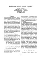
Figure 1: Probability densities for the accuracy
of the frequency method (dotted line) and the
smoothed log-linear model (solid line) on the mor-
phologically unrelated adjectives.
favorably with the resulting loss (gain) in residual
degrees of freedom. Using a fixed training set, six
of the fourteen variables were selected for modeling
the morphologically unrelated adjectives. Frequency
was selected as the only component of the model for
the morphologically related ones.
We also examined the possibility of replacing some
variables in these models by smoothing cubic B-
splines (Wahba, 1990). The analysis of deviance for
this model indicated that for the morphologically
unrelated adjectives, one of the six selected variables
should be removed altogether and another should be
replaced by a smoothing spline.
7 Evaluation of the Complex
Predictors
For both decision trees and log-linear regression, we
repeatedly partitioned the data in each of the two

groups into equally sized training and testing sets,
constructed the predictors using the training sets,
and evaluated them on the testing sets. This pro-
cess was repeated 200 times, giving vectors of esti-
mates for the performance of the various methods.
The simple frequency test was also evaluated in each
testing set for comparison purposes. From these vec-
tors, we estimate the density of the distribution of
the scores for each method; Figure 1 gives these den-
sities for the frequency test and the log-linear model
with smoothing splines on the most difficult case,
the morphologically unrelated adjectives.
Table 3 summarizes the performance of the meth-
ods on the two groups of adjective pairs. 4 In order
to assess the significance of the differences between
4The applicability of all complex methods was 100%
in both groups.
the scores, we performed a nonparametric sign test
(Gibbons and Chakraborti, 1992) for each complex
predictor against the simple frequency variable. The
test statistic is the number of runs where the score
of one predictor is higher than the other's; as is com-
mon in statistical practice, ties are broken by assign-
ing half of them to each category. Under the null
hypothesis of equal performance of the two methods
that are contrasted, this test statistic follows the bi-
nomial distribution with p = 0.5. Table 3 includes
the exact probabilities for obtaining the observed (or
more extreme) values of the test statistic.
From the table, we observe that the tree-based

methods perform considerably worse than frequency
(significant at any conceivable level), even when
cross-validation is employed. Both the standard
and smoothed log-linear models outperform the fre-
quency test on the morphologically unrelated adjec-
tives (significant at the 5% and 0.1% levels respec-
tively), while the log-linear model's performance is
comparable to the frequency test's on the morpho-
logically related adjectives. The best predictor over-
all is the smoothed log-linear model. 5
The above results indicate that the frequency test
essentially contains almost all the information that
can be extracted collectively from all linguistic tests.
Consequently, even very sophisticated methods for
combining the tests can offer only small improve-
ment. Furthermore, the prominence of one variable
can easily lead to overfitting the training data in the
remaining variables. This causes the decision tree
models to perform badly.
8 Conclusions and Future Work
We have presented a quantitative analysis of the per-
formance of measurable linguistic tests for the selec-
tion of the semantically unmarked term out of a pair
of antonymous adjectives. The analysis shows that a
simple test, word frequency, outperforms more com-
plicated tests, and also dominates them in terms of
information content. Some of the tests that have
been proposed in the linguistics literature, notably
tests that are based on the formal complexity and
differentiation properties of the words; fail to give

any useful information at all, at least with the ap-
proximations we used for them (Section 3). On the
other hand, tests based on morphological productiv-
ity are valid, although not as accurate as frequency.
Naturally, the validity of our results depends on
the quality of our measurements. While for most of
the variables our measurements are necessarily ap-
sit should be noted here that the independence as-
sumption of the sign test is mildly violated in these re-
peated runs, since the scores depend on collections of in-
dependent samples from a
finite
population. This mild
dependence will increase somewhat the probabilities un-
der the true null distribution, but we can be confident
that probabilities such as 0.08% will remain significant.
202
Morphologically Morphologically Overall
Predictor tested unrelated related
Accuracy P-Value Accuracy P-Value Accuracy P-Value
Frequency 75.87% - 97.15% - 81.07% -
Decision tree
(no cross-validation) 64.99% 8.2.10 -53 94.40% 1.5.10 -l° 72.05% 1.7- 10 TM
Decision tree 10-40 75.19% 7.2.10 -47
(cross validated) 69.13% 94.40% 1.5- 10 -l°
Log-linear model
(no smoothing) 76.52% 0.0281 97.17% 1.00 81.55% 0.0228
Log-linear model
(with smoothing) 76.82% 0.0008 97.17% 1.00 81.77% 0.0008
Table 3: Evaluation of the complex predictors. The probability of obtaining by chance a difference in

performance relative to the simple frequency test equal to or larger than the observed one is listed in the
P- Value
column for each complex predictor.
proximate, we believe that they are nevertheless of
acceptable accuracy since (1) we used a representa-
tive corpus; (2) we selected both a large sample of
adjective pairs and a large number of frequent ad-
jectives to avoid sparse data problems; (3) the pro-
cedure of identifying secondary words for indirect
measurements based on morphological productivity
operates with high recall and precision; and (4) the
mapping of the linguistic tests to comparisons of
quantitative variables was in most cases straightfor-
ward, and always at least plausible.
The analysis of the linguistic tests and their com-
binations has also led to a computational method
for the determination of semantic markedness. The
method is completely automatic and produces ac-
curate results at 82% of the cases. We consider
this performance reasonably good, especially since
no previous automatic method for the task has been
proposed. While we used a fixed set of 449 adjec-
tives for our analysis, the number of adjectives in
unrestricted text is much higher, as we noted in Sec-
tion 2. This multitude of adjectives, combined with
the dependence of semantic markedness on the do-
main, makes the manual identification of markedness
values impractical.
In the future, we plan to expand our analy-
sis to other classes of antonymous words, particu-

larly verbs which are notoriously difficult to ana-
lyze semantically (Levin, 1993). A similar method-
ology can be applied to identify unmarked (posi-
tive) versus marked (negative) terms in pairs such
as agree: dissent.
Acknowledgements
This work was supported jointly by the Advanced
Research Projects Agency and the Office of Naval
Research under contract N00014-89-J-1782, and by
the National Science Foundation under contract
GER-90-24069. It was conducted under the auspices
of the Columbia University CAT in High Perfor-
mance Computing and Communications in Health-
care, a New York State Center for Advanced Tech-
nology supported by the New York State Science and
Technology Foundation. We wish to thank Judith
Klavans, Rebecca Passonneau, and the anonymous
reviewers for providing us with useful comments on
earlier versions of the paper.
References
R. J. Baker and J. A. Nelder. 1989.
The
GLIM
System, Release 3: Generalized Linear Interactive
Modeling.
Numerical Algorithms Group, Oxford.
Edwin L. Battistella. 1990.
Markedness: The Eval-
uative Superstructure of Language.
State Univer-

sity of New York Press, Albany, NY.
T. Boucher and C. E. Osgood. 1969. The Polyanna
hypothesis.
Journal of Verbal Learning and Verbal
Behavior,
8:1-8.
Leo Breiman, J. H. Friedman, R. Olshen, and C. J.
Stone. 1984.
Classification and Regression Trees.
Wadsworth International Group, Belmont, CA.
M. Coltheart. 1981. The MRC Psycholinguis-
tic Database.
Quarterly Journal of Experimental
Psychology,
33A:497-505.
James Deese. 1964. The associative structure of
some common English adjectives.
Journal of Ver-
bal Learning and Verbal Behavior,
3(5):347-357.
Richard O. Duda and Peter E. Hart. 1973.
Pattern
Classification and Scene Analysis.
Wiley, New
York.
Jean Dickinson Gibbons and Subhabrata Chak-
raborti. 1992.
Nonparametric Statistical Infer-
ence.
Marcel Dekker, New York, 3rd edition.

203
Joseph H. Greenberg. 1966. Language Universals.
Mouton, The Hague.
Gregory Grefenstette. 1992. Finding semantic simi-
larity in raw text: The Deese antonyms. In Prob-
abilistic Approaches to Natural Language: Papers
from the 1992 Fall Symposium. AAAI.
T. Hastie and D. Pregibon. 1990. Shrinking trees.
Technical report, AT&T Bell Laboratories.
Vasileios Hatzivassiloglou and Kathleen McKeown.
1993. Towards the automatic identification of ad-
jectival scales: Clustering adjectives according to
meaning. In Proceedings of the 31st Annual Meet-
ing of the ACL, pages 172-182, Columbus, Ohio.
Roman Jakobson. 1962. Phonological Studies, vol-
ume 1 of Selected Writings. Mouton, The Hague.
Roman Jakobson. 1984a. The structure of the Rus-
sian verb (1932). In Russian and Slavic Grammar
Studies 1931-1981, pages 1-14. Mouton, Berlin.
Roman Jakobson. 1984b. Zero sign (1939). In
Russian and Slavic Grammar Studies 1931-1981,
pages 151-160. Mouton, Berlin.
John S. Justeson and Slava M. Katz. 1991. Co-
occurrences of antonymous adjectives and their
contexts. Computational Linguistics, 17(1):1-19.
Kevin Knight and Steve K. Luk. 1994. Building
a large-scale knowledge base for machine transla-
tion. In Proceedings of the 12th National Confer-
ence on Artificial Intelligence (AAAI-94). AAAI.
Henry KuSera and Winthrop N. Francis. 1967.

Computational Analysis of Present-Day American
English. Brown University Press, Providence, RI.
Henry Ku6era. 1982. Markedness and frequency:
A computational analysis. In Jan Horecky, edi-
tor, Proceedings of the Ninth International Con-
ference on Computational Linguistics (COLING-
82), pages 167-173, Prague. North-Holland.
George Lakoff. 1987. Women, Fire, and Dangerous
Things. University of Chicago Press, Chicago.
Adrienne Lehrer. 1985. Markedness and antonymy.
Journal of Linguistics, 31(3):397-429, September.
Beth Levin. 1993. English Verb Classes and Alter-
nations: A Preliminary Investigation. University
of Chicago Press, Chicago.
Stephen C. Levinson. 1983. Pragmatics. Cambridge
University Press, Cambridge, England.
John Lyons. 1977. Semantics, volume 1. Cambridge
University Press, Cambridge, England.
Peter McCullagh and John A. Nelder. 1989. Gen-
eralized Linear Models. Chapman and Hall, Lon-
don, 2nd edition.
Igor A. Mel'~uk and Nikolaj V. Pertsov. 1987. Sur-
face Syntax of English: a Formal Model within
the Meaning-Text Framework. Benjamins, Ams-
terdam and Philadelphia.
George A. Miller, R. Beckwith, C. Fellbaum,
D. Gross, and K. J. Miller. 1990. WordNet: An
on-line lexical database. International Journal of
Lexicography (special issue), 3(4):235-312.
John R. Quinlan. 1986. Induction of decision trees.

Machine Learning, 1(1):81-106.
Randolph Quirk, Sidney Greenbaum, Geoffrey
Leech, and Jan Svartvik. 1985. A Comprehensive
Grammar of the English Language. Longman,
London and New York.
Philip Resnik. 1993. Semantic classes and syntactic
ambiguity. In Proceedings of the ARPA Workshop
on Human Language Technology. ARPA Informa-
tion Science and Technology Office.
John R. Ross. 1987. Islands and syntactic pro-
totypes. In B. Need et ah, editors, Papers
from the 23rd Annual Regional Meeting of the
Chicago Linguistic Society (Part I: The General
Session), pages 309-320. Chicago Linguistic Soci-
ety, Chicago.
Thomas J. Santner and Diane E. Duffy. 1989. The
Statistical Analysis of Discrete Data. Springer-
Verlag, New York.
John Sinclair (editor in chief). 1987. Collins
COBUILD English Language Dictionary. Collins,
London.
Frank Smadja. 1993. Retrieving collocations
from text: XTRACT. Computational Linguistics,
19(1):143-177, March.
Nikolai S. Trubetzkoy. 1939. Grundzuger der
Phonologic. Travaux du Cercle Linguistique de
Prague 7, Prague. English translation in (Trubet-
zkoy, 1969).
Nikolai S. Trubetzkoy. 1969. Principles of Phonol-
ogy. University of California Press, Berkeley and

Los Angeles, California. Translated into English
from (Trubetzkoy, 1939).
Grace Wahba. 1990. Spline Models for Observa-
tional Data. CBMS-NSF Regional Conference se-
ries in Applied Mathematics. Society for Indus-
trial and Applied Mathematics (SIAM), Philadel-
phia, PA.
Linda R. Waugh. 1982. Marked and unmarked: A
choice between unequals. Semiotica, 38:299-318.
Margaret Winters. 1990. Toward a theory of syn-
tactic prototypes. In Savas L. Tsohatzidis, editor,
Meanings and Prototypes: Studies in Linguistic
Categorization, pages 285-307. Routledge, Lon-
don.
George K. Zipf. 1949. Human Behavior and the
Principle of Least Effort: An Introduction to Hu-
man Ecology. Addison-Wesley, Reading, MA.
A. Zwicky. 1978. On markedness in morphology.
Die Spra'che, 24:129-142.
204