Báo cáo khoa học: "Combining Distributional and Morphological Information for Part of Speech Induction" doc

Combining Distributional and Morphological Information for Part of
Speech Induction
Alexander Clark
ISSCO / TIM
University of Geneva
UNI-MAIL, Boulevard du Pont-d'Arve,
CH-1211 Geneve 4,
Switzerland

Abstract
In this paper we discuss algorithms for
clustering words into classes from un-
labelled text using unsupervised algo-
rithms, based on distributional and mor-
phological information. We show how
the use of morphological information
can improve the performance on rare
words, and that this is robust across a
wide range of languages.
1 Introduction
The task studied in this paper is the unsupervised
learning of parts-of-speech, that is to say lexical
categories corresponding to traditional notions of,
for example, nouns and verbs. As is often the case
in machine learning of natural language, there are
two parallel motivations: first a simple engineer-
ing one — the induction of these categories can
help in smoothing and generalising other mod-
els, particularly in language modelling for speech
recognition as explored by (Ney et al., 1994) and
secondly a cognitive science motivation — explor-

ing how evidence in the primary linguistic data
can account for first language acquisition by in-
fant children (Finch and Chater, 1992a; Finch and
Chater, 1992b; Redington et al., 1998). At this
early phase of learning, only limited sources of
information can be used: primarily distributional
evidence, about the contexts in which words oc-
cur, and morphological evidence, (more strictly
phonotactic or orthotactic evidence) about the se-
quence of symbols (letters or phonemes) of which
each word is formed. A number of different ap-
proaches have been presented for this task using
exclusively distributional evidence to cluster the
words together, starting with (Lamb, 1961) and
these have been shown to produce good results in
English, Japanese and Chinese. These languages
have however rather simple morphology and thus
words will tend to have higher frequency than in
more morphologically complex languages.
In this paper we will address two issues: first,
whether the existing algorithms work adequately
on a range of languages and secondly how we can
incorporate morphological information. We are
particularly interested in rare words: as (Rosen-
feld, 2000, pp.1313-1314) points out, it is most
important to cluster the infrequent words, as we
will have reliable information about the frequent
words; and yet it is these words that are most dif-
ficult to cluster. We accordingly focus both in our
algorithms and our evaluation on how to cluster

words effectively that occur only a few times (or
not at all) in the training data. In addition we are
interested primarily in inducing small numbers of
clusters (at most 128) from comparatively small
amounts of data using limited or no sources of
external knowledge, and in approaches that will
work across a wide range of languages, rather than
inducing large numbers (say 1000) from hundreds
of millions of words. Note this is different from
the common task of guessing the word category
of an unknown word given a pre-existing set of
parts-of-speech, a task which has been studied ex-
tensively (Mikheev, 1997).
Our approach will be to incorporate morpholog-
59
ical information of a restricted form into a distri-
butional clustering algorithm. In addition we will
use a very limited sort of frequency information,
since rare words tend to belong to open class cate-
gories. The input to the algorithm is a sequence of
tokens, each of which is considered as a sequence
of characters in a standard encoding.
The rest of this paper is structured as follows:
we will first discuss the evaluation of the models
in some detail and present some simple experi-
ments we have performed here (Section 2). We
will then discuss the basic algorithm that is the
starting point for our research in Section 3. Then
we show how we can incorporate a limited form
of morphological information into this algorithm

in Section 4. Section 5 presents the results of our
evaluations on a number of data sets drawn from
typologically distinct languages. We then briefly
discuss the use of ambiguous models or soft clus-
tering in Section 6, and then finish with our con-
clusions and proposals for future work.
2 Evaluation Discussion
A number of different approaches to evaluation
have been proposed in the past. First, early work
used an informal evaluation of manually compar-
ing the clusters or dendrograms produced by the
algorithms with the authors' intuitive judgment of
the lexical categories. This is inadequate for a
number of obvious reasons — first it does not al-
low adequate comparison of different techniques,
and secondly it restricts the languages that can
easily be studied to those in which the researcher
has competence thus limiting experimentation on
a narrow range of languages.
A second form of evaluation is to use some data
that has been manually or semi-automatically an-
notated with part of speech (POS) tags, and to use
some information theoretic measure to look at the
correlation between the 'correct' data and the in-
duced POS tags. Specifically, one could look at
the conditional entropy of the gold standard tags
given the induced tags. We use the symbol W to
refer to the random variable related to the word,
G
for the associated gold standard tag, and

T
for the
tag produced by one of our algorithms. Recall that
H(CT) = H(C) — I (G;T)
Thus low conditional entropy means that the
mutual information between the gold and induced
tags will be high. If we have a random set of tags
the mutual information will be zero and the con-
ditional entropy will be the same as the entropy of
the tag set.
Again, this approach has several weaknesses:
there is not a unique well-defined set of part-of-
speech tags, but rather many different possible sets
that reflect rather arbitrary decisions by the anno-
tators. To put the scores we present below in con-
text, we note that using some data sets prepared for
the AMALGAM project (Atwell et al., 2000) the
conditional entropies between some data manually
tagged with different tag sets varied from 0.22 (be-
tween Brown and LOB tag sets) to 1.3 (between
LLC and Unix Parts tag sets). Secondly, because
of the Zipfian distribution of word frequencies,
simple baselines that assign each frequent word
to a different class, can score rather highly, as we
shall see below.
A third evaluation is to use the derived clas-
sification in a class-based language model, and
to measure the perplexity of the derived model.
However it is not clear that this directly measures
the linguistic plausibility of the classification. In

particular many parts of speech (relative pronouns
for example) represent long-distance
combinato-
rial properties, and a simple finite-state model
with local context (such as a class n-gram model
(Brown et al., 1992)) will not measure this.
We can also compare various simple baselines,
to see how they perform according to these simple
measures.
Frequent word baseline take the n — 1 most fre-
quent words and assign them each to a sepa-
rate class, and put all remaining words in the
remaining class.
Word baseline each word is in its own class.
We performed experiments on parts of the Wall
Street Journal corpus, using the corpus tags. We
chose sections 0 — 19, a total of about 500,000
words. Table 1 shows that the residual conditional
entropy with the word baseline is only 0.12. This
reflects lexical ambiguity. If all of the words were
unambiguous, then the conditional entropy of the
60
Data
n
H(CT)
H(TG)
Frequent
16
2.00 0.28
Frequent

32
1.75
0.49
Frequent
64
1.46
0.69
Frequent
128 1.25
0.95
Words
31102 0.12
4.28
Table 1: Comparison of different baseline
tag given the word would be zero. We are there-
fore justified in ignoring ambiguity for the mo-
ment, since it vastly improves the efficiency of the
algorithms. Clearly as the number of clusters in-
creases, the conditional entropy will decrease, as
is demonstrated below.
3 Basic algorithm
The basic methods here have been studied in de-
tail by (Ney et al., 1994), (Martin et al., 1998) and
(Brown et al., 1992).
We assume a vocabulary of words V =
{W
1
, }. Our task is to learn a determinis-
tic clustering, that is to say a class membership
function

g
from V into the set of class labels
, n}. This clustering can be used to de-
fine a number of simple statistical models. The
objective function we try to maximise will be the
likelihood of some model — i.e. the probability
of the data with respect to the model. The sim-
plest candidate for the model is the class bigram
model, though the approach can also be extended
to class trigram models. Suppose we have a corpus
of length
N, , wN.
We can assume an ad-
ditional sentence boundary token. Then the class
bigram model defines the probability of the next
word given the history as
P(wi
IOC
'
) =
P(wilg(wi))P(9(wi-1)1g(wi-2))
It is not computationally feasible to search
through all possible partitions of the vocabulary
to find the one with the highest value of the like-
lihood; we must therefore use some search algo-
rithm that will give us a local optimum. We follow
(Ney et al., 1994; Martin et al., 1998) and use an
exchange algorithm similar to the k-means algo-
rithm for clustering. This algorithm iteratively im-
proves the likelihood of a given clustering by mov-

ing each word from its current cluster to the cluster
that will give the maximum increase in likelihood,
or leaving it in its original cluster if no improve-
ment can be found. There are a number of dif-
ferent ways in which the initial clustering can be
chosen; it has been found, and our own experi-
ments have tended to confirm this, that the initial-
isation method has little effect on the final quality
of the clusters but can have a marked effect on the
speed of convergence of the algorithm. A more
important variation for our purposes is how the
rare words are treated. (Martin et al., 1998) leave
all words with a frequency of less than 5 in a par-
ticular class, from which they may not be moved.
4 Morphology
The second sort of information is information
about the sequence of letters or phones that form
each word. To take a trivial example, if we en-
counter an unknown word, say £212,000 then
merely looking at the sequence of characters that
compose it is enough to enable us to make a good
guess as to its part of speech. Less trivially, if a
word in English ends in -ing, then it is quite likely
to be a present participle.
We can distinguish this sort of information,
which perhaps could better be called orthotactic or
phonotactic information from a richer sort which
incorporates relational information between the
words — thus given a novel word that ends in "ing"
such as "derailing" one could use the information

that we had already seen the token "derailed" as
additional evidence.
One way to incorporate this simple source of in-
formation would be to use a mixture of string mod-
els alone, without distributional evidence. Some
preliminary experiments not reported here estab-
lished that this approach could only separate out
the most basic differences, such as sequences of
numbers.
4.1 Combined models
A more powerful approach is to combine the dis-
tributional information with the morphological in-
formation by composing the Ney-Essen clustering
model with a model for the morphology within a
Bayesian framework. We use the same formula for
61
the probability of the data given the model, but in-
clude an additional term for the probability of the
model, that depends on the strings used in each
cluster. We wish to bias the algorithm so that it
will put words that are morphologically similar in
the same cluster. We can consider thus a genera-
tive process that produces sets of clusters as used
before. Consider the vocabulary V to be a subset
of E* where E is the set of characters or phonemes
used, and let the model have for each cluster i a
distribution over E* say P. Then we define the
probability of the partition (the prior) as
P(g)=ft
H


(w)

(1)
i=1
g(w)=i
ignoring irrelevant normalisation constants. This
will give a higher probability to partitions where
morphologically similar strings are in the same
cluster. The models we will use here for the clus-
ter dependent word string probabilities will be let-
ter Hidden Markov Models (HMMs). We decided
to use HMMs rather than more powerful mod-
els, such as character trigram models, because we
wanted models that were capable of modelling
properties of the whole string; though in English
and in other European languages, local statistics
such as those used by n-gram models are ade-
quate to capture most morphological regularities,
in other languages this is not the case. Moreover,
we wish to have comparatively weak models oth-
erwise the algorithm will capture irrelevant ortho-
tactic regularities — such as a class of words start-
ing with "st" in English.
4.2 Frequency
In addition we can modify this to incorporate in-
formation about frequency. We know that rare
words are more likely to be nouns, proper nouns
or members of some other open word class rather
than say pronouns or articles. We can do this sim-

ply by adding prior class probabilities ai to the
above equation giving
P(g)
=
H
H
ce,Pi(w)

(2)
i=1
g(w)=i
We can use the maximum likelihood estimates
for
ozi
which are just the number of distinct types
in cluster i, divided by the total number of types in
the corpus. This just has the effect of discriminat-
ing between classes that will have lots of types (i.e.
open class clusters) and clusters that tend to have
few types (corresponding to closed class words).
It is possible that in some languages there might
be more subtle category related frequency effects,
that could benefit from more complex models of
frequency.
5 Evaluation
5.1 Cross-linguistic Evaluation
We used texts prepared for the MULTEXT-East
project (Erjavec and Ide, 1998) which consists of
data (George Orwell's novel
1984)

in seven lan-
guages: the original English together with Roma-
nian, Czech, Slovene, Bulgarian, Estonian, and
Hungarian. These are summarised in Table 2.
As can be seen they cover a wide range of lan-
guage families; furthermore Bulgarian is writ-
ten in Cyrillic, which slightly stretches the range.
Token-type ratios range from 12.1 for English to
4.84 for Hungarian. The tags used are extremely
fine-grained, and incorporate a great deal of infor-
mation about case, gender and so on — in Hun-
garian for example 400 tags are used with 86 tags
used only once.
Table 3 shows the result of our cross-linguistic
evaluation on this data. Since the data sets are so
small we decided to use the conditional entropy
evaluation. Here DO refers to the distributional
clustering algorithm where all words are clustered;
D5 leaves all words with frequency at most 5 in a
seperate cluster, DM uses morphological informa-
tion as well, DF uses frequency information and
DMF uses morphological and frequency informa-
tion. We evaluated it for all words, and also for
words with frequency at most 5. We can see that
the use of morphological information consistently
improves the results on the rare words by a sub-
stantial margin. In some cases, however, a simpler
algorithm performs better when all the words are
considered — notably in Slovene and Estonian.
5.2 Perplexity Evaluation

We have also evaluated this method by comparing
the perplexity of a class-based language model de-
62
Conditional entropy vs. exact frequency
2.4
2.2
2
1.8
1.6
>-
5
-
1.4
1.2
1
0.8
0.6
0.4
2

4

6

8

10

12


14

16

18

20
Frequency
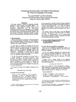
Figure 1: Graph showing performance of the six techniques on the WSJ data with 64 clusters. The
plot shows the conditional entropy of the gold standard tags given the cluster tags, for words of varying
frequencies.
Table 2: Data sets from Multext East Project
Language
Family
Tokens Types
Token/Type
Hapaxes
Tags
H (G)
H (G1W
)
English Germanic
118327
9771
12.1
4600
136
3.37
0.16
Bulgarian

Slavonic
101075
16352
6.2
9836
116
3.62
0.10
Czech
Slavonic 95828
19117
5.0
12048
956
4.41
0.21
Estonian
Finn-Ugrik
90452
17844
5.1
11643
404
3.92
0.14
Hungarian
Finn-Ugrik
98336
20321 4.8
13485

400
3.42
0.04
Romanian Romance
118289
14806
8.0 8088
581
4.03
0.10
Slovene Slavonic
107660
17868
6.0
10939
1033
4.34 0.20
Table 3: Cross-linguistic evaluation: 64 clusters, left all words, right
f <
5. We compare the baseline
with algorithms using purely distributional
(D)
evidence, supplemented with morphological (M) and
frequency (F) information.
H (G1C)
Base
DO
D5
D+M
D+F D+M+F

Base
DO
D+M
D+F D+M+F
All words
f <
5
English
1.52
0.98 0.95
1.00
0.97
0.94
2.33
1.53
1.20
1.51
1.16
Bulgarian 2.12
1.69
1.55
1.56
1.63
1.53
3.67
2.86 2.48
2.86
2.57
Czech
2.93

2.64 2.27
2.35
2.60
2.31
4.55
3.87
3.22
3.88
3.31
Estonian
2.44
2.31
1.88
2.12 2.29 2.09
4.01
3.42
3.14
3.42
3.14
Hungarian
2.16
2.04
1.76 1.80 2.01
1.70
4.07 3.46
3.06
3.40
3.18
Romanian
2.26

1.74
1.53
1.57
1.61
1.49 3.66
2.52
2.20
2.63 2.22
Slovene
2.60
2.28 2.01 2.08
2.21
2.07
4.59
3.72
3.25
3.73
3.55
63
Table 4: Perplexities on training data (left) and test
data(right) using WSJ data
Clusters
32
64
128
32
64
128
Training Test Data
Baseline

854
760
673
890
795
711
DO
479 380
316
692
585
529
D5
502 417
355
556 469 412
DF
484
386
325
652
516
462
DM
494 406
335
620
523
464
DMF

495
392
338 553
462
409
rived from these classes. We constructed a class
bigram model, using absolute interpolation with
a singleton generalised distribution for the transi-
tion weights, and using absolute discounting with
backing off for the membership/output function.
(Ney et al., 1994; Martin et al., 1998) We trained
the model on sections 00-09 of the Penn Tree-
bank, ( 518769 tokens including sentence bound-
aries and punctuation) and tested it on sections 10—
l 9 (537639 tokens). We used the full vocabulary
of the training and test sets together which was
45679, of which 14576 had frequency zero in the
training data and thus had to be categorised based
solely on their morphology and frequency. We did
not reduce the vocabulary or change the capital-
ization in any way. We compared different models
with varying numbers of clusters: 32 64 and 128.
Table 4 shows the results of the perplexity eval-
uation on the WSJ data. As can be seen the mod-
els incorporating morphological information have
slightly lower perplexity on the test data than the
D5 model. Note that this is a
global
evaluation
over all the words in the data, including words that

do not occur in the training data at all. Figure 5
shows how the conditional entropy varies with re-
spect to the frequency for these models. As can
be seen the use of morphological information im-
proves the preformance markedly for rare words,
and that this effect reduces as the frequency in-
creases. Note that the use of the frequency in-
formation worsens
the performance for rare words
according to this evaluation — this is because the
rare words are much more tightly grouped into just
a few clusters, thus the entropy of the cluster tags
is lower.
Table 5 shows a qualitative evaluation of some
of the clusters produced by the best performing
model for 64 clusters on the WSJ data set. We
selected the 10 clusters with the largest number of
zero frequency word types in. We examined each
cluster and chose a simple regular expression to
describe it, and calculated the precision and recall
for words of all frequency, and for words of zero
frequency. Note that several of the clusters cap-
ture syntactically salient morphological regulari-
ties: regular verb suffixes, noun suffixes and the
presence of capitalisation are all detected, together
with a class for numbers. In some cases these
are split amongst more than one class, thus giv-
ing classes with high precision and low recall. We
made no attempt to adjust the regular expressions
to make these scores high — we merely present

them as an aid to an intuitive understanding of the
composition of these clusters.
6 Ambiguous models
Up until now we have considered only
hard
clus-
ters, where each word is unambiguously assigned
to a single class. Clearly, because of lexical am-
biguity, we would like to be able to assign some
words to more than one class. This is sometimes
called
soft
clustering. Space does not permit an
extensive analysis of the situation. We shall there-
fore report briefly on some experiments we have
performed and our conclusions largely leaving this
as an area for future research.
(Jardino and Adda, 1994; Schiitze, 1997; Clark,
2000) have presented models that account for am-
biguity to some extent. The most principled way is
to use Hidden Markov Models: these provide the
formal and technical apparatus required to train
when the tags might be ambiguous. (Murakami
et al., 1993) presents this idea together with a
simple evaluation on English. We therefore ex-
tend our approach to allow ambiguous words, by
changing our model from a deterministic to non-
deterministic model. In this situation we want
the states of the HMM to correspond to syntac-
tic categories, and use the standard Expectation-

Maximization (EM) algorithm to train it.
To experiment with this we chose fully-
connected, randomly initialized Hidden Markov
Models, with determined start and end states. We
trained the model on the various sentences in the
64
Cluster Description
Regex
n
no
P
R
P
o
R
o
48
Capitalised words
[A-Z] [-a-z]+$
4396
1878 95
34
95
42
0
Numbers
\d+ [-\ .

] \d+$
4221

1843
99
86
98
86
33
Past tense verbs
ed$
3014
890
81
69
85
72
3
s suffix
s$
3351
873
62
40
63
40
28
lower case word
[-a-z1+$
2824
830
100
11

100
12
15
Capitalised words
[A-Z] [-a-z]+$
2539
776
95
20 94
17
60
present participles
ing$
2390
760
99
78
99
87
20
Capitalised words
[A-Z] [-a-z]+$
1723
756
99
14
100
18
51
lower case word

[-a-z1+$
2629
649
100
11
100
10
35
ALL CAPS
[A-Z1 *$
765
438
94
57
94
69
Table 5: The 10 most productive classes together with a qualitative analysis of their contents
Table 6: Evaluation of the pure HMM model, on
WSJ data G represents the gold standard tags, W
the word, and T the state of the HMM.
States
H(G1T)
H (T1W)
16
2.18
0.86
32
1.80
1.09
64

1.67
1.28
128
1.72
1.49
States
H(G1T)
H(TIW)
16
1.80
0.098
32
1.42
0.13
64
1.20
0.17
Table 7: Evaluation of the pure two-level HMM
model, on WSJ data. With 5 substates, 20 itera-
tions
corpus, and then tagged the data with the most
likely (Viterbi) tag sequence. We then evaluated
the conditional entropy of the gold standard tags
given the derived HMM tags.
Table 6 shows the results of this evaluation on
some English data for various numbers of states.
As can be seen, increasing the number of states
of the model does not reduce the conditional en-
tropy of the gold standard tags; rather it
increases

the lexical ambiguity of the model
H(TIW).
This
is because the states of the HMM will not neces-
sarily correspond directly to syntactic categories
— rather they correspond to sets of words that oc-
cur in particular positions — for example the model
might have a state that corresponds to a noun that
occurs before a main verb, and a separate state that
corresponds to a noun after a main verb. One ex-
planation for this is that the output function from
each state of the HMM is a multinomial distri-
bution over the vocabulary which is too power-
ful since it can memorise any set of words — thus
there is no penalty for the same word being pro-
duced by many different states. This suggests a
solution that is to replace the multinomial distri-
bution by a weaker distribution such as the Hidden
Markov Models we have used before. This gives
us a two-level HMM: a HMM where each state
corresponds to a word, and where the output func-
tion is a HMM where each state corresponds to a
letter. This relates to two other approaches that we
are aware of (Fine et al., 1998) and (Weber et al.,
2001).
Table 7 shows a simple evaluation of this ap-
proach; we can see that this does not suffer
from the same drawback as the previous approach
though the results are still poor compared to the
other approaches, and in fact are consistently

worse than the baselines of Table
1.
The problem
here is that we are restricted to using quite small
HMMs which are insufficiently powerful to mem-
orise large chunks of the vocabulary, and in addi-
tion the use of the Forward-Backward algorithm
is more computationally expensive — by at least a
factor of the number of states.
65
7 Conclusion
We have applied several different algorithms to
the task of identifying parts of speech. We have
demonstrated that the use of morphological infor-
mation can improve the performance of the algo-
rithm with rare words quite substantially. We have
also demonstrated that a very simple use of fre-
quency can provide further improvements. Addi-
tionally we have tested this on a wide range of lan-
guages. Intuitively we have used all of the differ-
ent types of information available - when we en-
counter a new word, we know three things about
it: first, the context that it has appeared in, sec-
ondly the string of characters that it is made of,
and thirdly that it is a new word and therefore rare.
7.1 Future work
We have so far used only a limited form of mor-
phological information that relies on properties of
individual strings, and does not relate particular
strings to each other. We plan to use this stronger

form of information using Pair Hidden Markov
Models as described in (Clark, 2001).
References
E. Atwell, G. Demetriou, J. Hughes, A. Schiffrin,
C. Souter, and S. Wilcock. 2000. A comparative
evaluation of modern English corpus grammatical
annotation schemes.
ICAME Journal,
24:7-23.
Peter F. Brown, Vincent J. Della Pietra, Peter V.
de Souza, Jenifer C. Lai, and Robert Mercer. 1992.
Class-based n-gram models of natural language.
Computational Linguistics, 18:467-479.
Alexander Clark. 2000. Inducing syntactic cate-
gories by context distribution clustering. In
Proc. of
CoNLL-2000 and LLL-2000,
pages 91-94, Lisbon,
Portugal.
Alexander Clark. 2001. Partially supervised learning
of morphology with stochastic transducers. In
Proc.
of Natural Language Processing Pacific Rim Sympo-
sium, NLPRS 2001,
pages 341-348, Tokyo, Japan,
November.
Toma'Z Erjavec and Nancy Ide. 1998. The MULTEXT-
East corpus. In
First International Conference
on Language Resources and Evaluation, LREC'98,

pages 971-974, Granada. ELRA.
S. Finch and N. Chater. 1992a. Bootstrapping syn-
tactic categories. In
Proceedings of the 14th An-
nual Meeting of the Cognitive Science Society,
pages
820-825.
S. Finch and N. Chater. 1992b. Bootstrapping syntac-
tic categories using statistical methods. In W. Daele-
mans and D. Powers, editors,
Background and Ex-
periments in Machine Learning of Natural Lan-
guage,
pages 229-235. Tilburg University: Institute
for Language Technology and Al.
Shai Fine, Yoram Singer, and Naftali Tishby. 1998.
The hierarchical Hidden Markov Model: Analysis
and applications.
Machine Learning,
32:41.
M. Jardino and G. Adda. 1994. Automatic determina-
tion of a stochastic bi-gram class language model. In
R. C. Carrasco and J. Oncina, editors, Grammatical
Inference and Applications: ICGI-94,
pages 57-65.
Springer-Verlag.
Sydney M. Lamb. 1961. On the mechanisation of
syntactic analysis. In
1961 Conference on Machine
Translation of Languages and Applied Language

Analysis,
volume 2, pages 674-685. HMSO, Lon-
don.
Sven Martin, JOrg Liermann, and Hermann Ney. 1998.
Algorithms for bigram and trigram word clustering.
Speech Communication,
24:19-37.
Andrei Mikheev. 1997. Automatic rule induction for
unknown word-guessing.
Computational Linguis-
tics,
23(3):405-423, September.
J.
Murakami, H. Yamatomo, and S. Sagayama. 1993.
The possibility for acquisition of statistical network
grammar using ergodic HMM. In
Proceedings of
Eurospeech 93, pages 1327-1330.
Hermann Ney, Ute Essen, and Reinhard Kneser.
1994. On structuring probabilistic dependencies in
stochastic language modelling.
Computer Speech
and Language, 8:1-38.
Martin Redington, Nick Chater, and Steven Finch.
1998. Distributional information: A powerful cue
for acquiring syntactic categories.
Cognitive Sci-
ence,
22(4):425-469.
Ronald Rosenfeld. 2000. Two decades of statistical

language modeling: Where do we go from here?
Proceedings of the IEEE,
88(8).
Hinrich Schtitze. 1997.
Ambiguity Resolution in Lan-
guage Learning.
CSLI Publications.
K.
Weber, S. Bengio, and H. Bourlard. 2001. Speech
recognition using advanced hmm2 features. IDIAP-
RR 24, IDIAP, Martigny, Switzerland. Published:
ASRU 2001, Madonna di Campiglio, Italy, Decem-
ber 2001.
66