Báo cáo khoa học: "Document Classification Using a Finite Mixture Model" pdf
Bạn đang xem bản rút gọn của tài liệu. Xem và tải ngay bản đầy đủ của tài liệu tại đây (750 KB, 9 trang )
Document Classification Using a Finite Mixture Model
Hang Li Kenji Yamanishi
C&C Res. Labs., NEC
4-1-1 Miyazaki Miyamae-ku Kawasaki, 216, Japan
Email: {lihang,yamanisi} @sbl.cl.nec.co.j p
Abstract
We propose a new method of classifying
documents into categories. We define for
each category a
finite mixture model
based
on
soft clustering
of words. We treat the
problem of classifying documents as that
of conducting statistical hypothesis testing
over finite mixture models, and employ the
EM algorithm to efficiently estimate pa-
rameters in a finite mixture model. Exper-
imental results indicate that our method
outperforms existing methods.
1 Introduction
We are concerned here with the issue of classifying
documents into categories. More precisely, we begin
with a number of categories (e.g., 'tennis, soccer,
skiing'), each already containing certain documents.
Our goal is to determine into which categories newly
given documents ought to be assigned, and to do so
on the basis of the distribution of each document's
words. 1
Many methods have been proposed to address
this issue, and a number of them have proved to
be quite effective (e.g.,(Apte, Damerau, and Weiss,
1994; Cohen and Singer, 1996; Lewis, 1992; Lewis
and Ringuette, 1994; Lewis et al., 1996; Schutze,
Hull, and Pedersen, 1995; Yang and Chute, 1994)).
The simple method of conducting hypothesis testing
over word-based distributions in categories (defined
in Section 2) is not efficient in storage and suffers
from the
data sparseness problem,
i.e., the number
of parameters in the distributions is large and the
data size is not sufficiently large for accurately es-
timating them. In order to address this difficulty,
(Guthrie, Walker, and Guthrie, 1994) have proposed
using distributions based on what we refer to as
hard
1A related issue is the retrieval, from a data base, of
documents which are relevant to a given query (pseudo-
document) (e.g.,(Deerwester et al., 1990; Fuhr, 1989;
Robertson and Jones, 1976; Salton and McGill, 1983;
Wong and Yao, 1989)).
clustering
of words, i.e., in which a word is assigned
to a single cluster and words in the same cluster are
treated uniformly. The use of hard clustering might,
however, degrade classification results, since the dis-
tributions it employs are not always precise enough
for representing the differences between categories.
We propose here to employ
soft chsterinf,
i.e.,
a word can be assigned to several different clusters
and each cluster is characterized by a specific word
probability distribution. We define for each cate-
gory a
finite mixture model,
which is a linear com-
bination of the word probability distributions of the
clusters. We thereby treat the problem of classify-
ing documents as that of conducting statistical hy-
pothesis testing over finite mixture models. In or-
der to accomplish hypothesis testing, we employ the
EM algorithm to efficiently and approximately cal-
culate from training data the maximum likelihood
estimates of parameters in a finite mixture model.
Our method overcomes the major drawbacks of
the method using word-based distributions and the
method based on hard clustering, while retaining
their merits; it in fact includes those two methods
as special cases. Experimental results indicate that
our method outperforrrLs them.
Although the finite mixture model has already
been used elsewhere in natural language processing
(e.g. (Jelinek and Mercer, 1980; Pereira, Tishby,
and Lee, 1993)), this is the first work, to the best of
knowledge, that uses it in the context of document
classification.
2 Previous Work
Word-based method
A simple approach to document classification is to
view this problem as that of conducting hypothesis
testing over word-based distributions. In this paper,
we refer to this approach as the
word-based method
(hereafter, referred to as WBM).
2We borrow from (Pereira, Tishby, and Lee, 1993)
the terms hard clustering and soft clustering, which were
used there in a different task.
39
Letting W denote a vocabulary (a set of words),
and w denote a random variable representing any
word in it, for each category
ci
(i = 1, ,n), we
define its
word-based distribution P(wIci)
as a his-
togram type of distribution over W. (The num-
ber of free parameters of such a distribution is thus
I W[-
1). WBM then views a document as a sequence
of words:
d = Wl,''" , W N
(1)
and assumes that each word is generated indepen-
dently according to a probability distribution of a
category. It then calculates the probability of a doc-
ument with respect to a category as
N
P(dlc,) = P(w,, ,~Nle,)
=
1-~ P(w, lc,), (2)
t=l
and classifies the document into that category for
which the calculated probability is the largest. We
should note here that a document's probability with
respect to each category is equivMent to the
likeli-
hood
of each category with respect to the document,
and to classify the document into the category for
which it has the largest probability is equivalent to
classifying it into the category having the largest
likelihood with respect to it. Hereafter, we will use
only the term likelihood and denote it as
L(dlci).
Notice that in practice the parameters in a dis-
tribution must be estimated from training data. In
the case of WBM, the number of parameters is large;
the training data size, however, is usually not suffi-
ciently large for accurately estimating them. This
is the
data .sparseness problem
that so often stands
in the way of reliable statistical language processing
(e.g.(Gale and Church, 1990)). Moreover, the num-
ber of parameters in word-based distributions is too
large to be efficiently stored.
Method based on hard clustering
In order to address the above difficulty, Guthrie
et.al, have proposed a method based on hard cluster-
ing of words (Guthrie, Walker, and Guthrie, 1994)
(hereafter we will refer to this method as HCM). Let
cl, ,c,~ be categories. HCM first conducts hard
clustering of words. Specifically, it (a) defines a vo-
cabulary as a set of words W and defines as clusters
its subsets kl, ,k,n satisfying
t3~=xk j = W
and
ki fq kj = 0 (i •
j)
(i.e., each word is assigned only
to a single cluster); and (b) treats uniformly all the
words assigned to the same cluster. HCM then de-
fines for each category
ci
a distribution of the clus-
ters
P(kj [ci) (j = 1, ,m).
It replaces each word
wt in the document with the cluster
kt
to which it
belongs (t = 1, , N). It assumes that a cluster
kt
is distributed according to
P(kj[ci)
and calculates
the likelihood of each category
ci
with respect to
the document by
N
L(dle,)
L(kl, , kNlci) = H e(k, le,).
t=l
(3)
Table 1: Frequencies of words
racket stroke shot goal kick ball
cl 4 1 2 1 0 2
c2 0 0 0 3 2 2
Table 2: Clusters and words (L = 5,M = 5)
' kl racket, stroke, shot
ks kick
. k 3 goal, ball
Table 3: Frequencies of clusters
kl ks k3
c 1 7 0 3
c2 0 2 5
There are any number of ways to create clusters in
hard clustering, but the method employed is crucial
to the accuracy of document classification. Guthrie
et. al. have devised a way suitable to documentation
classification. Suppose that there are two categories
cl ='tennis' and c2='soccer,' and we obtain from the
training data (previously classified documents) the
frequencies of words in each category, such as those
in Tab. 1. Letting L and M be given positive inte-
gers, HCM creates three clusters: kl, k2 and k3, in
which kl contains those words which are among the
L most frequent words in cl, and not among the M
most frequent in c2; k2 contains those words which
are among the L most frequent words in cs, and
not among the M most frequent in Cl; and k3 con-
tains all remaining words (see Tab. 2). HCM then
counts the frequencies of clusters in each category
(see Tab. 3) and estimates the probabilities of clus-
ters being in each category (see Tab. 4). 3 Suppose
that a newly given document, like d in Fig. i, is to
be classified. HCM cMculates the likelihood values
3We calculate the probabilities here by using the so-
called expected likelihood estimator (Gale and Church,
1990):
.f(kjlc, ) + 0.5 ,
P(k3lc~) = f-~ ~-~ x m
(4)
where
f(kjlci )
is the frequency of the cluster kj in ci,
f(ci) is the total frequency of clusters in
cl,
and m is the
total number of clusters.
40
Table 4: Probability distributions of clusters
kl k2 k3
cl 0.65 0.04 0.30
cs 0.06 0.29 0.65
L(dlCl )
and
L(dlc2)
according to Eq. (3). (Tab. 5
shows the logarithms of the resulting likelihood val-
ues.) It then classifies d into cs, as log s
L(dlcs )
is
larger than log s
L(dlc 1).
d = kick, goal, goal, ball
Figure 1: Example document
Table 5: Calculating log likelihood values
log2
L(dlct )
= 1 x log s .04 + 3 × log s .30 = -9.85
log s
L(d]cs)
= 1 × log s .29 + 3 x log s .65 = -3.65
HCM can handle the data sparseness problem
quite well. By assigning words to clusters, it can
drastically reduce the number of parameters to be
estimated. It can also save space for storing knowl-
edge. We argue, however, that the use of hard clus-
tering still has the following two problems:
1. HCM cannot assign a word ¢0 more than one
cluster at a time.
Suppose that there is another
category c3 = 'skiing' in which the word 'ball'
does not appear, i.e., 'ball' will be indicative of
both cl and c2, but not cs. If we could assign
'ball' to both kt and k2, the likelihood value for
classifying a document containing that word to
cl or c2 would become larger, and that for clas-
sifying it into c3 would become smaller. HCM,
however, cannot do that.
2. HCM cannot make the best use of information
about the differences among the frequencies of
words assigned to an individual cluster.
For ex-
ample, it treats 'racket' and 'shot' uniformly be-
cause they are assigned to the same cluster kt
(see Tab. 5). 'Racket' may, however, be more
indicative of Cl than 'shot,' because it appears
more frequently in cl than 'shot.' HCM fails
to utilize this information. This problem will
become more serious when the values L and M
in word clustering are large, which renders the
clustering itself relatively meaningless.
From the perspective of number of parameters,
HCM employs models having very few parameters,
and thus may not sometimes represent much useful
information for classification.
3 Finite Mixture Model
We propose a method of document classification
based on soft clustering of words. Let cl, ,cn
be categories. We first conduct the soft cluster-
ing. Specifically, we (a) define a vocabulary as a
set W of words and define as clusters a number of
its subsets kl, , k,n satisfying
u'~=lk j
= W; (no-
tice that
ki t3 kj = 0 (i ~ j)
does not necessarily
hold here, i.e., a word can be assigned to several dif-
ferent clusters); and (b) define for each cluster kj
(j = 1, , m) a distribution
Q(w[kj)
over its words
()"]~wekj Q(w[kj)
= 1) and a distribution
P(wlkj)
satisfying:
! Q(wlki); wek i,
P(wlkj)
0; w ¢ (5)
where w denotes a random variable representing any
word in the vocabulary. We then define for each cat-
egory
ci (i =
1, , n) a distribution of the clusters
P(kj Ici),
and define for each category a linear com-
bination of
P(w]kj):
P(wlc~)
= ~
P(kjlc~) x P(wlk.i) (6)
j=l
as the distribution over its words, which is referred
to as
afinite mixture model(e.g.,
(Everitt and Hand,
1981)).
We treat the problem of classifying a document
as that of conducting the likelihood ratio test over
finite mixture models. That is, we view a document
as a sequence of words,
d= wl, " " , WN
(7)
where
wt(t =
1, ,N) represents a word. We
assume that each word is independently generated
according to an unknown probability distribution
and determine which of the finite mixture mod-
els
P(w[ci)(i = 1, ,n)
is more likely to be the
probability distribution by observing the sequence of
words. Specifically, we calculate the likelihood value
for each category with respect to the document by:
L(d[ci) = L(wl, ,wglci)
= I-[~=1 P(wtlc,)
: n =l P(k ic,) x P(w, lk ))
(8)
We then classify it into the category having the
largest likelihood value with respect to it. Hereafter,
we will refer to this method as FMM.
FMM includes WBM and HCM as its special
cases. If we consider the specific case (1) in which
a word is assigned to a single cluster and
P(wlkj)
is
given by
{1.
(9)
P(wlkj)= O; w~k~,
41
where Ikjl denotes the number of elements belonging
to kj, then we will get the same classification result
as in HCM. In such a case, the likelihood value for
each category ci becomes:
L(dlc,) = I-I;:x (P(ktlci) x
P~wtlkt))
= 1-It=~ P(ktlci) x l-It=lP(Wtlkt),
(lo)
where kt is the cluster corresponding to
wt.
Since
the probability
P(wt]kt)
does not depend on eate-
N
gories, we can ignore the second term YIt=l
P(wt Ikt)
in hypothesis testing, and thus our method essen-
tially becomes equivalent to HCM (c.f. Eq. (3)).
Further, in the specific case (2) in which m = n,
for each
j,
P(wlkj)
has IWl parameters:
P(wlkj)
=
P(wlcj),
and
P(kjlci )
is given by
1; i = j,
P(kjlci)=
O; i#j,
(11)
the likelihood used in hypothesis testing becomes
the same as that in Eq.(2), and thus our method
becomes equivalent to WBM.
4 Estimation and Hypothesis
Testing
In this section, we describe how to implement our
method.
Creating clusters
There are any number of ways to create clusters on a
given set of words. As in the case of hard clustering,
the way that clusters are created is crucial to the
reliability of document classification. Here we give
one example approach to cluster creation.
Table 6: Clusters and words
Ikl Iracket, stroke, shot, balll
ks kick, goal, ball
We let the number of clusters equal that of cat-
egories (i.e., m = n) 4 and relate each cluster ki
to one category ci (i = 1, ,n). We then assign
individual words to those clusters in whose related
categories they most frequently appear. Letting 7
(0 _< 7 < 1) be a predetermined threshold value, if
the following inequality holds:
f(wlci)
> 7, (t2)
f(w)
then we assign w to ki, the cluster related to ci,
where
f(wlci)
denotes the frequency of the word w
in category ci, and
f(w)
denotes the total frequency
ofw. Using the data in Tab.l, we create two clusters:
kt and k2, and relate them to ct and c2, respectively.
4One can certainly assume that m > n.
For example, when 7 = 0.4, we assign 'goal' to k2
only, as the relative frequency of 'goal' in c~ is 0.75
and that in cx is only 0.25. We ignore in document
classification those words which cannot be assigned
to any cluster using this method, because they are
not indicative of any specific category. (For example,
when 7 >_ 0.5 'ball' will not be assigned into any
cluster.) This helps to make classification efficient
and accurate. Tab. 6 shows the results of creating
clusters.
Estimating
P(wlk j)
We then consider the frequency of a word in a clus-
ter. If a word is assigned only to one cluster, we view
its total frequency as its frequency within that clus-
ter. For example, because 'goal' is assigned only to
ks, we use as its frequency within that cluster the to-
tal count of its occurrence in all categories. If a word
is assigned to several different clusters, we distribute
its total frequency among those clusters in propor-
tion to the frequency with which the word appears
in each of their respective related categories. For
example, because 'ball' is assigned to both kl and
k2, we distribute its total frequency among the two
clusters in proportion to the frequency with which
'ball' appears in cl and c2, respectively. After that,
we obtain the frequencies of words in each cluster as
shown in Tab. 7.
Table 7: Distributed frequencies of words
racket stroke shot goal kick ball
kl 4 1 2 0 0 2
k2 0 0 0 4 2 2
We then estimate the probabilities of words in
each cluster, obtaining the results in Tab. 8. 5
Table 8: Probability distributions of words
racket stroke shot goal kick ball
kl 0.44 0.11 0.22 0 0 0.22
k2 0 0 0 0.50 0.25 0.25
Estimating
P( kj ]ci)
Let us next consider the estimation of
P(kj[ci).
There are two common methods for statistical esti-
mation, the maximum likelihood estimation method
5We calculate the probabilities by employing the
maximum likelihood estimator:
/(kAc0 (13)
P(kilci)- f(ci) '
where
f(kj]cl)
is the frequency of the cluster kj in ci,
and
f(cl)
is the total frequency of clusters in el.
42
Table 10: Calculating log likelihood values
[log~L(d[cl)=
log2(.14× .25)+2x log2(.14x .50)+log2(.86x.22 +.14x .25): -14.67[
I
log S
L(dlc2 )
1og2(.96 x .25) + 2 x log2(.96 x .50) + 1og2(.04 x .22 T .96 × .25) -6.18 I
Table 9: Probability distributions of clusters
kl k2
Cl 0.86 0.14
c2 0.04 0.96
and the Bayes estimation method. In their imple-
mentation for estimating
P(kj Ici),
however, both of
them suffer from computational intractability. The
EM algorithm (Dempster, Laird, and Rubin, 1977)
can be used to efficiently approximate the maximum
likelihood estimator of
P(kj
[c~). We employ here an
extended version of the EM algorithm (Helmbold et
al., 1995). (We have also devised, on the basis of
the Markov chain Monte Carlo (MCMC) technique
(e.g. (Tanner and Wong, 1987; Yamanishi, 1996)) 6,
an algorithm to efficiently approximate the Bayes
estimator of
P(kj
[c~).)
For the sake of notational simplicity, for a fixed i,
let us write
P(kjlci) as Oj
and
P(wlkj) as Pj(w).
Then letting 9 = (01,'",0m), the finite mixture
model in Eq. (6) may be written as
rn
P(wlO) = ~0~ x
Pj(w).
(14)
j=l
For a given training sequence
wl'"WN,
the maxi-
mum likelihood estimator of 0 is defined as the value
which maximizes the following log likelihood func-
tion
)
L(O)
= ~'log OjPj(wt)
.
(15)
~- \j=l
The EM algorithm first arbitrarily sets the initial
value of 0, which we denote as 0(0), and then suc-
cessively calculates the values of 6 on the basis of its
most recent values. Let s be a predetermined num-
ber. At the lth iteration (l -: 1, , s), we calculate
=
by
0~ '): 0~ '-1) (~?(VL(00-1))j- 1)+ 1), (16)
where ~ > 0 (when ~ = 1, Hembold et al. 's version
simply becomes the standard EM algorithm), and
6We have confirmed in our preliminary experiment
that MCMC performs slightly better than EM in docu-
ment classification, but we omit the details here due to
space limitations.
~TL(O)
denotes
v L(O) = ( 0L001 "'" O0,nOL )
. (17)
After s numbers of calculations, the EM algorithm
outputs 00) = (0~O, ,0~ )) as an approximate of
0. It is theoretically guaranteed that the EM al-
gorithm converges to a local minimum of the given
likelihood (Dempster, Laird, and Rubin, 1977).
For the example in Tab. 1, we obtain the results
as shown in Tab. 9.
Testing
For the example in Tab. 1, we can calculate ac-
cording to Eq. (8) the likelihood values of the two
categories with respect to the document in Fig. 1
(Tab. 10 shows the logarithms of the likelihood val-
ues). We then classify the document into category
c2, as log 2
L(d]c2)
is larger than log 2
L(dlcl).
5 Advantages of FMM
For a probabilistic approach to document classifica-
tion, the most important thing is to determine what
kind of probability model (distribution) to employ
as a representation of a category. It must (1) ap-
propriately represent a category, as well as (2) have
a proper preciseness in terms of number of param-
eters. The goodness and badness of selection of a
model directly affects classification results.
The finite mixture model we propose is particu-
larly well-suited to the representation of a category.
Described in linguistic terms, a cluster corresponds
to a
topic
and the words assigned to it are related
to that topic. Though documents generally concen-
trate on a single topic, they may sometimes refer
for a time to others, and while a document is dis-
cussing any one topic, it will naturally tend to use
words strongly related to that topic. A document in
the category of 'tennis' is more likely to discuss the
topic of 'tennis,' i.e., to use words strongly related
to 'tennis,' but it may sometimes briefly shift to the
topic of 'soccer,' i.e., use words strongly related to
'soccer.' A human can follow the sequence of words
in such a document, associate them with related top-
ics, and use the distributions of topics to classify the
document. Thus the use of the finite mixture model
can be considered as a stochastic implementation of
this process.
The use of FMM is also appropriate from the
viewpoint of number of parameters. Tab. 11 shows
the numbers of parameters in our method (FMM),
43
Table 11: Num. of parameters
WBM O(n. IWl)
HCM O(n. m)
FMM
o(Ikl+n'm)
HCM, and WBM, where IW] is the size of a vocab-
ulary,
Ikl
is the sum of the sizes of word clusters
m
(i.e.,Ikl E~=I Ikil), n is the number of categories,
and m is the number of clusters. The number of
parameters in FMM is much smaller than that in
WBM, which depends on
IWl,
a very large num-
ber in practice (notice that
Ikl
is always smaller
than
IWI
when we employ the clustering method
(with 7 > 0.5) described in Section 4. As a result,
FMM requires less data for parameter estimation
than WBM and thus can handle the data sparseness
problem quite well. Furthermore, it can economize
on the space necessary for storing knowledge. On
the other hand, the number of parameters in FMM
is larger than that in HCM. It is able to represent the
differences between categories more precisely than
HCM, and thus is able to resolve the two problems,
described in Section 2, which plague HCM.
Another advantage of our method may be seen in
contrast to the use of latent semantic analysis (Deer-
wester et al., 1990) in document classification and
document retrieval. They claim that their method
can solve the following problems:
synonymy problem how to group synonyms, like
'stroke' and 'shot,' and make each relatively
strongly indicative of a category even though
some may individually appear in the category
only very rarely;
polysemy problem how to determine that a word
like 'ball' in a document refers to a 'tennis ball'
and not a 'soccer ball,' so as to classify the doc-
ument more accurately;
dependence problem how to use de-
pendent words, like 'kick' and 'goal,' to make
their combined appearance in a document more
indicative of a category.
As seen in Tab.6, our method also helps resolve all
of these problems.
6 Preliminary Experimental Results
In this section, we describe the results of the exper-
iments we have conducted to compare the perfor-
mance of our method with that of HCM and others.
As a first data set, we used a subset of the Reuters
newswire data prepared by Lewis, called Reuters-
21578 Distribution 1.0. 7 We selected nine overlap-
ping categories, i.e. in which a document may be-
rReuters-21578 is available at
long to several different categories. We adopted the
Lewis Split in the corpus to obtain the training data
and the test data. Tabs. 12 and 13 give the de-
tails. We did not conduct stemming, or use stop
words s. We then applied FMM, HCM, WBM , and
a method based on cosine-similarity, which we de-
note as COS 9, to conduct binary classification. In
particular, we learn the distribution for each cate-
gory and that for its complement category from the
training data, and then determine whether or not to
classify into each category the documents in the test
data. When applying FMM, we used our proposed
method of creating clusters in Section 4 and set 7
to be 0, 0.4, 0.5, 0.7, because these are representative
values. For HCM, we classified words in the same
way as in FMM and set 7 to be 0.5, 0.7, 0.9, 0.95.
(Notice that in HCM, 7 cannot be set less than 0.5.)
Table 12: The first data set
Num. of doc. in training data 707
Num. of doc in test data 228
Num. of (type of) words 10902
Avg. num. of words per doe. 310.6
Table 13: Categories in the first data set
I wheat,corn,oilseed,sugar,coffee
soybean,cocoa,rice,cotton ]
Table 14: The second data set
Num. of doc. training data 13625
Num. of doc. in test data 6188
Num. of (type of) words 50301
Avg. num. of words per doc. 181.3
As a second data set, we used the entire Reuters-
21578 data with the Lewis Split. Tab. 14 gives the
details. Again, we did not conduct stemming, or use
stop words. We then applied FMM, HCM, WBM ,
and COS to conduct binary classification. When ap-
plying FMM, we used our proposed method of creat-
ing clusters and set 7 to be 0, 0.4, 0.5, 0.7. For HCM,
we classified words in the same way as in FMM and
set 7 to be 0.5, 0.7, 0.9, 0.95. We have not fully com-
pleted these experiments, however, and here we only
8'Stop words' refers to a predetermined list of words
containing those which are considered not useful for doc-
ument classification, such as articles and prepositions.
9In this method, categories and documents to be clas-
sified are viewed as vectors of word frequencies, and the
cosine value between the two vectors reflects similarity
(Salton and McGill, 1983).
44
Table 15: Tested categories in the second data set
earn,acq,crude,money-fx,gr ain
interest,trade,ship,wheat,corn ]
give the results of classifying into the ten categories
having the greatest numbers of documents in the test
data (see Tab. 15).
For both data sets, we evaluated each method in
terms of
precision
and
recall
by means of the so-
called micro-averaging 10
When applying WBM, HCM, and FMM, rather
than use the standard likelihood ratio testing, we
used the following heuristics. For simplicity, suppose
that there are only two categories cl and c2. Letting
¢ be a given number larger than or equal 0, we assign
a new document d in the following way:
~
(logL(dlcl) -logL(dlc2))
> e; d * cl,
(logL(dlc2) logL(dlct)) > ~; d + cu,
otherwise; unclassify d,
(is)
where N is the size of document d. (One can easily
extend the method to cases with a greater ~umber of
categories.) 11 For COS, we conducted classification
in a similar way.
Fig s. 2 and 3 show precision-recall curves for the
first data set and those for the second data set, re-
spectively. In these graphs, values given after FMM
and HCM represent 3' in our clustering method (e.g.
FMM0.5, HCM0.5,etc). We adopted the break-even
point as a single measure for comparison, which is
the one at which precision equals recall; a higher
score for the break-even point indicates better per-
formance. Tab. 16 shows the break-even point for
each method for the first data set and Tab. 17 shows
that for the second data set. For the first data set,
FMM0 attains the highest score at break-even point;
for the second data set, FMM0.5 attains the highest.
We considered the following questions:
(1) The training data used in the experimen-
tation may be considered sparse. Will a word-
clustering-based method (FMM) outperform a word-
based method (WBM) here?
(2) Is it better to conduct soft clustering (FMM)
than to do hard clustering (HCM)?
(3) With our current method of creating clusters,
as the threshold 7 approaches 0, FMM behaves much
like WBM and it does not enjoy the effects of clus-
tering at all (the number of parameters is as large
l°In micro-averaging(Lewis and Ringuette, 1994), pre-
cision is defined as the percentage of classified documents
in all categories which are correctly classified. Recall is
defined as the percentage of the total documents in all
categories which are correctly classified.
nNotice that words which are discarded in the duster-
ing process should not to be counted in document size.
I
0.g
0.8
0.7
~ 0.6
0.5
0.4
0.3
0.2
~" _':~ "HCM0.S" -e
.~". ::.':. ~ °HCM0.7" v,
, " " ~ "'~"~ "HCMO.9" ~
.~/ - " "-~, "HCM0.g5" -~'
• ." ~, "., "FMM0" -e
/ ~. ~ "FMM0.4" "+
~ / '~ ~ ~ "FMM0.5" -e
y
-,,
"FMMO.7"
/.~::::~: ~
'-,.
, 1 : .
0.1 0.2 0.3 0.4 0.5 0.6 0.7 0.8 0.9
recall
Figure 2: Precision-recall curve for the first data set
c
I I
O.g
0.8
0.7
0.6
0,5
0.4
0.3
0.2
0.1
"WBM"
"+
"HCM0.5" -D-
"HCM0.7 = K
GI, "" "HCMO.g" ~
""'~- "HCMO.g5" "~ -
"'"'l~ ~3~
"FMMO" -e.
".
"~. ~ Q °FMM0.4" -+
• ,.:" ",,,. "FMM0.5" -Q
% " -,~ "FMM0.7 ~
" " ~, ~
°0, 012 0:~ 01, 0:s 0:0 0:, 0:8 01,
recall
Figure 3: Precision-recall curve for the second data
set
as in WBM). This is because in this case (a) a word
will be assigned into all of the clusters, (b) the dis-
tribution of words in each cluster will approach that
in the corresponding category in WBM, and (c) the
likelihood value for each category will approach that
in WBM (recall case (2) in Section 3). Since creating
clusters in an optimal way is difficult, when cluster-
ing does not improve performance we can at least
make FMM perform as well as WBM by choosing
7 = 0. The question now is "does FMM perform
better than WBM when 7 is 0?"
In looking into these issues, we found the follow-
ing:
(1) When 3' >> 0, i.e., when we conduct clustering,
FMM does not perform better than WBM for the
first data set, but it performs better than WBM for
the second data set.
Evaluating classification results on the basis of
each individual category, we have found that for
three of the nine categories in the first data set,
45
Table 16: Break-even point
COS
WBM
HCM0.5
HCM0.7
HCM0.9
HCM0.95
FMM0
FMM0.4
FMM0.5
FMM0.7
for thq first data set
0.60
0.62
0.32
0.42
0.54
0.51
0.66
0.54
0.52
0.42
Table 17: Break-even point for the
COS 10.52
WBM !0.62
HCM0.5 10.47
HCM0.7 i0.51
HCM0.9 10.55
HCM0.95 0.31
FMM0 i0.62
FMM0.4 0.54
FMM0.5 0.67
FMM0.7 0.62
second data set
FMM0.5 performs best, and that in two of the ten
categories in the second data set FMM0.5 performs
best. These results indicate that clustering some-
times does improve classification results
when we
use our current way of creating clusters.
(Fig. 4
shows the best result for each method for the cate-
gory 'corn' in the first data set and Fig. 5 that for
'grain' in the second data set.)
(2) When 3' >> 0, i.e., when we conduct clustering,
the best of FMM almost always outperforms that of
HCM.
(3) When 7 = 0, FMM performs better than
WBM for the first data set, and that it performs
as well as WBM for the second data set.
In summary, FMM always outperforms HCM; in
some cases it performs better than WBM; and in
general it performs at least as well as WBM.
For both data sets, the best FMM results are supe-
rior to those of COS throughout. This indicates that
the probabilistic approach is more suitable than the
cosine approach for document classification based on
word distributions.
Although we have not completed our experiments
on the entire Reuters data set, we found that the re-
sults with FMM on the second data set are almost as
good as those obtained by the other approaches re-
ported in (Lewis and Ringuette, 1994). (The results
are not directly comparable, because (a) the results
in (Lewis and Ringuette, 1994) were obtained from
an older version of the Reuters data; and (b) they
t
0,9
0.8
0.7
0.8
0.8
'COS"
"'~/ , "HCMO.9" ~
• '~ "~., "FMMO.8"
,/ "-~
o'., °'., o'.~ o'., o.~ oi° oi, o'.8 o'.8
ror,~
Figure 4: Precision-recall curve for category 'corn'
1
°.9
0.8
0.7
0,6
0.5
0.4
0.3
0.2
O.t
"" k~,
• ~
"h~MO.7"
"e ",
FMI¢~.$
I
0'., 0'., 0'., 0'., 0'.8 0'., 0., 0.° 01,
Figure 5: Precision-recall curve for category 'grain'
used stop words, but we did not.)
We have also conducted experiments on the Su-
sanne corpus data t2 and confirmed the effectiveness
of our method. We omit an explanation of this work
here due to space limitations.
7 Conclusions
Let us conclude this paper with the following re-
marks:
1. The primary contribution of this research is
that we have proposed the use of the finite mix-
ture model in document classification.
2. Experimental results indicate that our method
of using the finite mixture model outperforms
the method based on hard clustering of words.
3. Experimental results also indicate that in some
cases our method outperforms the word-based
12The Susanne corpus, which has four non-overlapping
categories, is ~va~lable at
46
method
when we use our current method of cre-
ating clusters.
Our future work is to include:
1. comparing the various methods over the entire
Reuters corpus and over other data bases,
2. developing better ways of creating clusters.
Our proposed method is not limited to document
classification; it can also be applied to other natu-
ral language processing tasks, like word sense dis-
ambiguation, in which we can view the context sur-
rounding a ambiguous target word as a document
and the word-senses to be resolved as categories.
Acknowledgements
We are grateful to Tomoyuki Fujita of NEC for his
constant encouragement. We also thank Naoki Abe
of NEC for his important suggestions, and Mark Pe-
tersen of Meiji Univ. for his help with the English of
this text. We would like to express special apprecia-
tion to the six ACL anonymous reviewers who have
provided many valuable comments and criticisms.
References
Apte, Chidanand, Fred Damerau, and Sholom M.
Weiss. 1994. Automated learning of decision rules
for text categorization.
A CM Tran. on Informa-
tion Systems,
12(3):233-251.
Cohen, William W. and Yoram Singer. 1996.
Context-sensitive learning methods for text cat-
egorization.
Proc. of SIGIR'96.
Deerwester, Scott, Susan T. Dumais, George W.
Furnas, Thomas K. Landauer, and Richard Harsh-
man. 1990. Indexing by latent semantic analysis.
Journ. of the American Society for Information
Science,
41(6):391-407.
Dempster, A.P., N.M. Laird, and D.B. Rubin. 1977.
Maximum likelihood from incomplete data via the
em algorithm.
Journ. of the Royal Statistical So-
ciety, Series B,
39(1):1-38.
Everitt, B. and D. Hand. 1981.
Finite Mixture Dis-
tributions.
London: Chapman and Hall.
Fuhr, Norbert. 1989. Models for retrieval with prob-
abilistic indexing.
Information Processing and
Management,
25(1):55-72.
Gale, Williams A. and Kenth W. Church. 1990.
Poor estimates of context are worse than none.
Proc. of the DARPA Speech and Natural Language
Workshop,
pages 283-287.
Guthrie, Louise, Elbert Walker, and Joe Guthrie.
1994. Document classification by machine: The-
ory and practice.
Proc. of COLING'94,
pages
1059-1063.
Helmbold, D., R. Schapire, Y. Siuger, and M. War-
muth. 1995. A comparison of new and old algo-
rithm for a mixture estimation problem.
Proc. of
COLT'95,
pages 61-68.
Jelinek, F. and R.I. Mercer. 1980. Interpolated esti-
mation of markov source parameters from sparse
data.
Proc. of Workshop on Pattern Recognition
in Practice,
pages 381-402.
Lewis, David D. 1992. An evaluation of phrasal and
clustered representations on a text categorization
task.
Proc. of SIGIR'9~,
pages 37-50.
Lewis, David D. and Marc Ringuette. 1994. A com-
parison of two learning algorithms for test catego-
rization.
Proc. of 3rd Annual Symposium on Doc-
ument Analysis and Information Retrieval,
pages
81-93.
Lewis, David D., Robert E. Schapire, James P.
Callan, and Ron Papka. 1996. Training algo-
rithms for linear text classifiers.
Proc. of SI-
GIR '96.
Pereira, Fernando, Naftali Tishby, and Lillian Lee.
1993. Distributional clustering of english words.
Proc. of ACL '93,
pages 183-190.
Robertson, S.E. and K. Sparck Jones. 1976. Rel-
evance weighting of search terms.
Journ. of
the American Society for Information Science,
27:129-146.
Salton, G. and M.J. McGiU. 1983.
Introduction to
Modern Information Retrieval.
New York: Mc-
Graw Hill.
Schutze, Hinrich, David A. Hull, and Jan O. Peder-
sen. 1995. A comparison of classifiers and doc-
ument representations for the routing problem.
Proc. of SIGIR '95.
Tanner, Martin A. and Wing Hung Wong. 1987.
The calculation of posterior distributions by data
augmentation.
Journ. of the American Statistical
Association,
82(398):528-540.
Wong, S.K.M. and Y.Y. Ya~. 1989. A probability
distribution model for information retrieval.
In-
formation Processing and Management,
25(1):39-
53.
Yamanishi, Kenji. 1996. A randomized approxima-
tion of the mdl for stochastic models with hidden
variables.
Proc. of COLT'96,
pages 99-109.
Yang, Yiming and Christoper G. Chute. 1994. An
example-based mapping method for text catego-
rization and retrieval.
A CM Tran. on Information
Systems,
12(3):252-277.
47