Identification of spatio temporal clusters of lung cancer cases in pennsylvania, usa 2010–2017
Bạn đang xem bản rút gọn của tài liệu. Xem và tải ngay bản đầy đủ của tài liệu tại đây (1.22 MB, 7 trang )
(2022) 22:555
Camiña et al. BMC Cancer
/>
Open Access
RESEARCH
Identification of spatio‑temporal clusters
of lung cancer cases in Pennsylvania, USA:
2010–2017
Nuria Camiña1,2, Tara L. McWilliams1,3, Thomas P. McKeon1,2,4, Trevor M. Penning1,2,5 and Wei‑Ting Hwang1,3,5,6*
Abstract
Background: It is known that geographic location plays a role in developing lung cancer. The objectives of this study
were to examine spatio-temporal patterns of lung cancer incidence in Pennsylvania, to identify geographic clusters of
high incidence, and to compare demographic characteristics and general physical and mental health characteristics
in those areas.
Method: We geocoded the residential addresses at the time of diagnosis for lung cancer cases in the Pennsylvania
Cancer Registry diagnosed between 2010 and 2017. Relative risks over the expected case counts at the census tract
level were estimated using a log-linear Poisson model that allowed for spatial and temporal effects. Spatio-temporal
clusters with high incidence were identified using scan statistics. Demographics obtained from the 2011–2015 Ameri‑
can Community Survey and health variables obtained from 2020 CDC PLACES database were compared between
census tracts that were part of clusters versus those that were not.
Results: Overall, the age-adjusted incidence rates and the relative risk of lung cancer decreased from 2010 to 2017
with no statistically significant space and time interaction. The analyses detected 5 statistically significant clusters over
the 8-year study period. Cluster 1, the most likely cluster, was in southeastern PA including Delaware, Montgomery,
and Philadelphia Counties from 2010 to 2013 (log likelihood ratio = 136.6); Cluster 2, the cluster with the largest area
was in southwestern PA in the same period including Allegheny, Fayette, Greene, Washington, and Westmoreland
Counties (log likelihood ratio = 78.6). Cluster 3 was in Mifflin County from 2014 to 2016 (log likelihood ratio = 25.3),
Cluster 4 was in Luzerne County from 2013 to 2016 (log likelihood ratio = 18.1), and Cluster 5 was in Dauphin, Cum‑
berland, and York Counties limited to 2010 to 2012 (log likelihood ratio = 17.9). Census tracts that were part of the
high incidence clusters tended to be densely populated, had higher percentages of African American and residents
that live below poverty line, and had poorer mental health and physical health when compared to the non-clusters
(all p < 0.001).
Conclusions: These high incidence areas for lung cancer warrant further monitoring for other individual and envi‑
ronmental risk factors and screening efforts so lung cancer cases can be identified early and more efficiently.
Keywords: Lung cancer, Incidence, Spatio-temporal, Geographic clustering, Scan statistics, Pennsylvania
*Correspondence:
6
Department of Biostatistics, Epidemiology and Informatics, Perelman School
of Medicine, University of Pennsylvania, Philadelphia, PA, USA
Full list of author information is available at the end of the article
Introduction
Lung cancer is the most frequently diagnosed cancer
worldwide, accounting for 1.74 million deaths annually
and lung cancer cases are expected to increase by 38% to
2.89 million by 2030 [1]. Lung cancer is also the leading
© The Author(s) 2022. Open Access This article is licensed under a Creative Commons Attribution 4.0 International License, which
permits use, sharing, adaptation, distribution and reproduction in any medium or format, as long as you give appropriate credit to the
original author(s) and the source, provide a link to the Creative Commons licence, and indicate if changes were made. The images or
other third party material in this article are included in the article’s Creative Commons licence, unless indicated otherwise in a credit line
to the material. If material is not included in the article’s Creative Commons licence and your intended use is not permitted by statutory
regulation or exceeds the permitted use, you will need to obtain permission directly from the copyright holder. To view a copy of this
licence, visit http://creativecommons.org/licenses/by/4.0/. The Creative Commons Public Domain Dedication waiver (http://creativeco
mmons.org/publicdomain/zero/1.0/) applies to the data made available in this article, unless otherwise stated in a credit line to the data.
Camiña et al. BMC Cancer
(2022) 22:555
cause of cancer mortality in both men and women in the
U.S. In 2021, Pennsylvania (PA) was ranked 32 out of 49
states with an age-adjusted lung cancer incidence rate of
63 per 100,000 population and a five-year survival rate
of 25 percent [2]. An estimated 5,990 Pennsylvanians are
expected to die from lung cancer in 2022 with approximately 11,170 new cases being reported [3]. People diagnosed at early stages of lung cancer are five times more
likely to survive; however, in Pennsylvania only 16 percent of lung cancer cases are diagnosed at early stages [2].
Documenting the extent of cancer incidence remains
central to improving public health research and to developing population-based strategies for cancer prevention.
The need to understand the incidence of lung cancer is
influenced by potentially modifiable risk factors (e.g.,
tobacco use, alcohol drinking, unhealthy diet, radon
exposure) and others that are not (e.g., inherited genetic
mutations) [3]. Cancer outcomes are influenced also by
socioeconomic status, access to care, supportive services,
and rural–urban environmental factors, all of which contribute to both the physical and mental health of cancer
patients [4].
Mapping spatial patterns of lung cancer risk is an
increasingly popular approach given the greater availability of geographically enabled cancer data and sophisticated visualization methods [5]. Maps are useful for
examining disease patterns in relation to local environmental factors with the ability to examine disease causation through the identification of demographic patterns
and trends [6, 7].
Spatial statistical methods like space–time models can
also be used to quantify patterns and trends over space
and time (i.e., spatio-temporal) and cancer clusters are
frequently used by researchers to respond to public concerns. The aims of this study were to examine spatio-temporal patterns of lung cancer incidence in Pennsylvania
over an 8-year period (2010–2017), identify high incidence clusters, and compare the demographic and health
characteristics of residents inside and outside of clusters.
Methods
Data sources
Lung and bronchus cancer cases in PA between 2010
and 2017 were obtained from the Pennsylvania Cancer
Registry (PCR) [8] using International Statistical Classification of Diseases, 10th revision (ICD 10) diagnosis
codes—C340 (main bronchus), C341 (upper lobe, bronchus or lung), C342 (middle lobe, bronchus or lung),
C343 (lower lobe, bronchus or lung), C348 (overlapping
sites of bronchus and lung), and C349 (unspecified part
of bronchus or lung). PCR is an incidence-based registry and has earned Gold Certification from the North
American Association of Central Cancer Registries
Page 2 of 12
(NAACCR), the highest level of data quality achieving at
least 95% completeness, for all years under study [9]. The
following three exclusion criteria were applied to exclude
cases that were: (i) in situ and non-carcinoma histology,
(ii) not uniquely matched with a census tract ID, and (iii)
the age of diagnosis belonged to an age group with zero
population size as estimated by US Census Bureau indicating a possible error. This resulted in a total of 73,937
cases from 3,197 census tracts. We used the census tract,
the small and relatively permanent statistical subdivision
defined by the US Census Bureau, as the unit of analysis for the consistency in the data collected over the years
and the validity when used in research studies [10]. We
conducted the present analysis under a data use agreement with the Pennsylvania Department of Health and
with the approval of the University of Pennsylvania Institutional Review Board (IRB number 831671).
The reported street addresses at the time of diagnosis
were geocoded using ArcGIS 10.6.1 software [11] and
matched with the 2010 census tract ID. Lung cancer cases
were grouped into 18 age groups (0–4, 5–9, 10–14,15–
19, 20–24, 25–29, 30–34, 35–39, 40–44, 45–49, 50–54,
55–59, 60–64, 65–74, 75–84, 85 and above). Annual population size for the same year by age groups for a census
tract was obtained using the American Community Survey (ACS), a national survey conducted by the US Census
Bureau that provides various individual demographic and
household information on a yearly basis [12].
Demographic data at the census tract level were
extracted from the 2011–2015 ACS including median
age (years), percentage of males, distribution by race and
ethnicity, per capita income, median household income
(thousands of $), percent poverty, distribution by educational attainment, total population size, and population
density (per square mile).
Poor mental health and poor physical health, defined
as the percent of individuals ≥ 18 years who self-reported
having 14 or more days during the past 30 days in which
their mental or physical health was not good, were
extracted from the Centers for Disease Control and Prevention (CDC) PLACES 2020 database derived using
the 2018 Behavioural Risk Factor Surveillance System
(BRFSS). Both mental and physical health measures
were based on self-assessment only without an objective
health component [13].
Age‑adjusted Incidence rates and trends over time
The age-adjusted incidence rates (number of cases per
100,000) for each census tract were calculated by adjusting the crude incidence rate with respect to the 2000 U.S.
Standard Million Population, a commonly used standard
population for adjustment that assumes a total population of 1,000,000 [14]. The adjustment used the 18 age
Camiña et al. BMC Cancer
(2022) 22:555
groups and population size estimates described above. A
choropleth map for the age-adjusted incidence rate using
the cumulative cases over 8 years was created to visualize the spatial pattern. Temporal trends in the adjusted
incidence rates were examined and modeled using linear
quantile mixed models [15]. Such mixed models were utilized to allow census tract level random effects of intercept and slope for the calendar year to be estimated,
while the use of the quantile regression provided a robust
summary of the trends that were less sensitive to outlying
values in the incidence rates, which are often observed in
smaller census tracts. The estimated 5
0th (median), 75th,
th
th
80 , and 90 quantiles were plotted, and the mean profile was included as a reference.
Spatio‑temporal disease risk and mapping
To understand the spatio-temporal disease risk, we modeled the observed case counts through a log-linear Poisson regression with both spatial and temporal terms, as
well as a space–time interaction term. Specifically, the
mean case count for location i (in this case a census tract)
and year j was modeled as the expected case counts for
the same location and year combination (Eij) times the
relative risk parameter, R
Rij, which is also indexed by
location i and year j (i.e., relative risk specific to a location and a time). The expected case counts E
ij were determined based on the age distribution of the corresponding
location i and year j such that Eij equals the crude incidence rate in a particular age group in the study population in year j times the population size in the same age
group of the location i from the same year (i.e., internal
standardization). Extending the model proposed by Lawson et al. [16] for the spatial model, the log of the space–
time relative risk parameter R
Rij was modeled with four
components: an intercept as the overall relative risk for
the study region, location-specific random effects, a
linear trend term in time j, and the interaction random
effects between the location and time. The spatial random effects were assumed to follow a normal distribution
under the conditional autoregressive (CAR) setting based
on Queen contiguity spatial weight matrix (i.e., two areas
are considered neighbors if they share a common boundary). The model was fit using the R-integrated nested
Laplace approximation, R-INLA [17] under the Bayesian
framework with a normal prior distribution. Temporal
trends in the RR estimates from 20 randomly selected
census tracts were plotted to examine the changes over
time. The spatial pattern for the estimated RR for a given
year was illustrated using a choropleth map. Furthermore, we calculated the standardized incidence ratio
(SIR) for each census tract as the total number of cases
observed divided by the total number of cases expected
Eij across the 8 years combined. We then created a
Page 3 of 12
choropleth map of the SIR to examine this spatial pattern empirically with SIR > 1 indicating an elevated risk
such that the number of cases observed is higher than the
expected number of cases.
Detection of high‑risk clusters
We used the SaTScan cluster detection method which
employs Kulldorff scan statistics to detect high risk clusters. This approach has been widely used in spatial statistics to evaluate the risk of disease geographically to detect
high risk clusters. This method generated circular spatial
windows of various sizes and evaluated the observed over
the expected number of cases by comparing inside versus outside the circles to identify statistically significant
clusters [18]. To detect spatio-temporal clusters [19, 20],
scan statistics covered the study area with many overlapping “windows” now defined as cylinders with the base as
the area and the height as the time period in the space–
time setting. As the window expanded to contain more
areas and more cases, we used a log-linear ratio (LLR) to
compare the number of cases inside the windows to the
number of cases outside the window. The null hypothesis was calculated under the probability that being a
case is the same inside and outside the window relative to
the age-adjusted expected number of cases. A LLR > > 1
indicated evidence that the current window forms a high
incidence or high-risk cluster. In our analysis, the ageadjusted expected case counts used were the same Eij that
was used for the log-linear Poisson model in the previous
section. The most likely cluster (i.e., the window with the
maximum LLR) and secondary clusters (i.e., other statistically significant windows at 0.05 significance level) were
identified in the current analysis. The RR of each cluster
was determined by the total number of cases observed
over the total number of cases expected in the years
when the cluster is present. The statistical significance of
a cluster was determined through a Monte Carlo hypothesis testing procedure [21]. The proposed analysis was
performed using the R shiny application SpatialEpiApp,
which allows estimation of spatio-temporal disease risk
and detection of clusters [22].
Comparison of census tracts in high‑risk cluster versus not
The nonparametric Wilcoxon rank sum test with a continuity correction was used to compare demographic
variables between census tracts in any high incidence
cluster at any time during 2010 to 2017 versus those not
in any clusters. Data on smoking, which is a known risk
factor for lung cancer development, were not available
at the census tract level and for the same time frame as
the demographic variables used, thus comparison of the
smoking prevalence between census tracts was not possible. A two-sided p < 0.01 was considered statistically
Camiña et al. BMC Cancer
(2022) 22:555
Page 4 of 12
significant. We used a lower p-value threshold for statistical significance to account for testing multiple variables.
Results
Age‑adjusted incidence rates and spatio‑temporal disease
risk
The population density by census tract in Pennsylvania using the 2011–2015 ACS is shown in Fig. 1A. The
population was mainly concentrated in a small number of
metropolitan areas including the southeast and western
regions of Pennsylvania, specifically in Philadelphia and
Pittsburgh areas, respectively. A map of age-adjusted
incidence rate using the cumulative cases over 8 years
is provided in Fig. 1B showing that higher age-adjusted
incidence rates were mainly observed in the major cities
located in southeastern (e.g., Philadelphia), northeastern
(e.g., Allentown, Scranton), and western (e.g., Pittsburgh,
Erie) Pennsylvania. The age-adjusted incidence rates
decreased slightly over the study period with median
incidence rates (25th-75th quantiles) of 51.7 per 100,000
(A)
0
50
100
150 km
N
Population Density
(per sq. mile)
2011−2015
100
300
500
1500
Pittsburgh
10000
Harrisburg
Philadelphia
67000
(B)
0
50
100
150 km
N
Age−Adjusted
Incidence Rate,
2010−2017
30
50
70
80
Pittsburgh
90
Harrisburg
252
Philadelphia
Fig. 1 A population density based on the 2011–2015 5-year ACS, B age-adjusted incidence rate based on the cumulative cases over 8 years from
2010 to 2017
(2022) 22:555
Page 5 of 12
150
(A)
50
100
90%−tile
80%−tile
75%−tile
mean
median (50%−tile)
0
Estimated quantiles and mean profiles
(rate per 100,000)
Camiña et al. BMC Cancer
2010 2011 2012 2013 2014 2015 2016 2017
Year
1.5
Relative Risk 2010
0.5
1.0
(0.156,0.802]
(0.802,0.885]
(0.885,0.944]
(0.944,0.992]
(0.992,1.05]
(1.05,1.1]
(1.1,1.17]
(1.17,1.24]
(1.24,1.34]
(1.34,1.5]
(1.5,2.88]
0.0
Average Relative Risk
(B)
2010 2011 2012 2013 2014 2015 2016 2017
Year
Fig. 2 A temporal trends in the estimated quantiles and mean profiles (rate per 100,000) from 2010 to 2017 based on the linear mixed quantile
regression model, B temporal trends in the average of the estimated RR from 2010 to 2017 based on the log-linear Poisson spatio-temporal model,
grouped by decile of 2010 estimates
(25.2 to 83.3) for 2010, 49.1 per 100,000 (24.4 to 78.9) for
2013, and 45.3 per 100,000 (22.0 to 72.3) for 2017, respectively, approximately 0.8 per 100,000 per year, for all the
quantiles and the mean values are shown in Fig. 2A.
The estimated relative risk (RR) from the log-linear
Poisson regression model suggested no statistically significant space and time interaction (p > 0.05) and revealed
a steady decrease in lung cancer incidence from 2010 to
2017. The median RR values (25th-75th quantiles) were
1.07 (0.93 to 1.26) for 2010, 1.01 (0.88 to 1.19) for 2013,
and 0.95 (0.82 to 1.12) for 2017, respectively. Figure 2B
shows the estimated RR over time for 20 randomly
selected census tracts and the median of RR estimates for
a decile group created using the 2010 estimates. The parallel lines observed in Fig. 2A and B reflected that the fitted models suggested no space and time interaction such
that the decreasing trends in the age-adjusted incidence
rates and RR values were consistent across the study
region. Maps showing the estimated RR for 2013 and SIR
are provided in Fig. 3A and B, respectively, indicating a
similar pattern to the age-adjusted incidence rates as
shown in Fig. 1B, such that higher values of RR and SIR
were concentrated in the major cities located in southeastern (e.g., Philadelphia), northeastern (e.g., Allentown,
Scranton) and western (e.g., Pittsburgh, Erie) Pennsylvania while most of the central PA showed lower than
expected case counts (RR < 1 and SIR < 1). Maps from
other years also show a similar pattern (maps not shown).
Detection of high‑risk clusters
Five spatio-temporal clusters were identified based on
lung cancer cases in Pennsylvania during the study period
2010 to 2017, as shown in Fig. 4. Information for each of
the clusters is provided in Table 1. The most likely cluster (Cluster 1), which is the cluster with the largest LLR,
was from 2010 to 2013 with a RR of 1.35. This cluster
with an average population size of 1,276,868 was in the
Philadelphia metropolitan area including the neighboring
Camiña et al. BMC Cancer
(2022) 22:555
Page 6 of 12
(A)
0
50
100
150 km
N
Relative Risk, 2013
0
0.75
1.25
3
Pittsburgh
Harrisburg
Philadelphia
(B)
0
50
100
150 km
N
SIR, 2010−2017
0
0.5
0.9
1.25
1.75
10
Pittsburgh
Harrisburg
Philadelphia
Fig. 3 A estimated RR for 2013 based on log-linear Poisson spatio-temporal model, B SIR based on the cumulative cases from over 8 years from
2010 to 2017
Delaware and Montgomery Counties, part of the southeastern PA. Among the four secondary clusters, one cluster (Cluster 2) from 2010 to 2013 with a RR of 1.22 was
in southwestern PA: Allegheny County, Fayette County,
Greene County, Washington County, and Westmoreland
County. This cluster had the highest number of observed
lung cancer cases reaching 4,601. Three other secondary clusters (Clusters 3 to 5) were identified for varying
periods: Cluster 3 was in Mifflin County in the central PA
from 2014 to 2016, associated with the smallest number
of individuals 3,772 on average, and observed a total of 30
cases while only 6 cases were expected; Cluster 4 was in
Luzerne County from 2013 to 2016 near the AllentownScranton region; lastly, Cluster 5 was in the southcentral
PA region near the Harrisburg area from 2010 to 2015
that included Dauphin, Cumberland, and York Counties.
It is important to note that the size of the area covered
by each cluster differed significantly, and the location and
Camiña et al. BMC Cancer
(2022) 22:555
Page 7 of 12
Fig. 4 Five spatio-temporal clusters in PA and the associated RRs and p-values. Cluster 3 shows Mifflin County; Cluster 1 Delaware, Montgomery,
and Philadelphia Counties; Cluster 2 Allegheny, Fayette, Greene, Washington, and Westmoreland Counties; Cluster 4 Luzerne County; and Cluster 5
Dauphin, Cumberland, and York Counties
the numbers of identified clusters also varied from one
time period to another. For example, as shown in Fig. 5,
there were three clusters (Clusters 1, 2, 5) from 2010 to
2012; three clusters (Clusters 1, 2, 4) in 2013, and two
clusters (Clusters 3 and 4) from 2014 to 2016. No clusters
were identified in 2017, the final year of the study period.
The demographic and health characteristics for the
identified five lung cancer clusters are provided in Table 2.
Significant differences were observed in median age, percent male, percent African American, per capita income,
percent poverty, percent high school graduate or higher,
population density, poor mental health, and poor physical health (all p < 0.001) between the clustered and nonclustered census tracts. In our analysis, census tracts that
were part of the high incidence clusters tended to have
residents of lower median age, had a higher percentage of
Table 1 Results of cluster analysis of lung cancer cases in Pennsylvania developed between 2010 and 2017
Cluster
Averaged
population
size
Years Detected
County
Observed cases
Expected cases
RR
LLR
1
1,276,868
2010–2013
Delaware, Montgomery and Philadelphia
3,557
2,676
1.4
136.6
2
1,260,363
2010–2013
Allegheny, Fayette, Greene, Washington
and Westmoreland
4,601
3,823
1.2
78.6
3
3,772
2014–2016
Mifflin
30
6
5.2
25.3
4
108,756
2013–2016
Luzerne
448
333
1.4
18.1
5
184,572
2010–2012
Dauphin, Cumberland and York
454
338
1.3
17.9