báo cáo hóa học: " Bayesian bias adjustments of the lung cancer SMR in a cohort of German carbon black production workers" pdf

RESEARC H Open Access
Bayesian bias adjustments of the lung cancer
SMR in a cohort of German carbon black
production workers
Peter Morfeld
1,2*
, Robert J McCunney
3
Abstract
Background: A German cohort study on 1,528 carbon black production workers estimated an elevated lung
cancer SMR ranging from 1.8-2.2 depending on the reference population. No positive trends with carbon black
exposures were noted in the analyses. A nested case control study, however, identified smoking and previous
exposures to known carcinogens, such as crystalline silica, received prior to work in the carbon black industry as
important risk factors.
We used a Bayesian procedure to adjust the SMR, based on a prior of seven independent parameter distributions
describing smoking behaviour and crystalline silica dust exposure (as indicator of a group of correlated carcinogen
exposures received previously) in the cohort and population as well as the strength of the relationship of these
factors with lung cancer mortality. We implemented the approach by Markov Chain Monte Carlo Methods (MCMC)
programmed in R, a statistical computing system freely available on the internet, and we provide the program
code.
Results: When putting a flat prior to the SMR a Markov chain of length 1,000,000 returned a median poste rior SMR
estimate (that is, the adjusted SMR) in the range between 1.32 (95% posterior interval: 0.7 , 2.1) and 1.00 (0.2, 3.3)
depending on the method of assessing previous exposures.
Conclusions: Bayesian bias adjustment is an excellent tool to effectively combine data about confounders from
different sources. The usually calculated lung cancer SMR statistic in a cohort of carbon black workers
overestimated effect and precision when compared with the Bayesian results. Quantitative bias adjustment should
become a regular tool in occupation al epidemiology to address narrative discussions of potential distortions.
Background
Carbon black is a powdered form of elemental carbon
that is ma nufactured by the controlled vapor-phase pyr-
olysis of hydrocarbons. Preferential raw materials for

most carbon black production processes are feedstock
oils that contain a high content of aromatic hydrocar-
bons. Over 90% of the world’s carbon black production
is used for the reinforcement of rubber; about two
thirds are used for tires and one third for the produc-
tion of technical rubber articles.
Car tires contain approximately 30% t o 35% of carbon
blacks of different types. The remaining world produc-
tion of carbon black is used for printing inks, colours
and lacquers, stabilizers for synthetics, and in the electri-
cal industry [1]. Currently, greater than 95% of worldwide
car bon black production is via the oil furnace black pro-
cess [2]. Different grades of carbon black are typically
produc ed by using different reactor designs and by vary-
ing the reactor temperatures and/or residence times [3].
The most recent evaluation of possible human cancer
risks due to carbon black exposure was performed by an
IARC (International Agency for Rese arch on Cancer)
Working Group in February 2006 [4]. The Working
Group identified lung can cer as the most important
endpoint to consider and exposures to workers at car-
bon black production sites as the most relevant for an
evaluation of risk. The group concluded that the human
evidence for carcinogenicity was inadequate.(IARC,
overall Group 2B).
* Correspondence:
1
Institute for Occupational Medicine of Cologne University/Germany
Full list of author information is available at the end of the article
Morfeld and McCunney Journal of Occupational Medicine and Toxicology 2010, 5:23

/>© 2010 Morfeld and McCunney; licensee BioMed Central Ltd. This is an Open Access article distributed under the terms of the Creative
Commons Attribution License ( which permits unrestricted use, distribution, and
reproduction in any medium, provided the original work is properly cited.
Among the key studies evaluated by IARC [4] was a
German investigation of 1,528 carbon black production
workers[5-7]. Based on 50 observed cases a lung cancer
SMR (standardized mortality ratio) of 2.18 (0.95-CI:
1.61, 2.87; national reference rates from West Germany;
CI = confidence interval) or 1.83 (0.95-CI: 1.34, 2.39;
state reference rates from North-Rhine Westphalia) was
estimated. Positive trends with carbon black exposures
were not observed in internal dose-response analyses
[6,7]. However, a nested case-control study [8] identified
smoking and previous exposures to known carcinogens
prior to work at the carbon black plant as important
risk factors. Due to correlations between previo us expo-
sures to carcinogens, crystalline silica exposure was used
as a surrogate for the group of occupational confoun-
ders experienced prior to work at the carbon black
plant (see Büchte and co-workers [8] for details). A sim-
ple sensitivity analysis concluded that these two factors
(smoking and previous exposures) may explain the
major part of the excess risk in lung cancer reported in
the original cohort analysis [5]. The IARC working
group raised concer ns as to whether the simple sensitiv-
ity analysis was appropriate for adjustment since the
findings were difficult to interpret. We thus now present
results from a Bayesian bias adjustment that addresses
deficiencies of the simple sensitivity analysis.
Customarily, confidence intervals estimate random

error, not other sources of uncertainty, such as con-
founding, selection bias and m easurement error. To
address t his additional uncertainty of an effect measure
simple sensitivity analyses, Monte Carlo sensitivity ana-
lyses (Probability Sensitivity Analyses) or Bayesian ana-
lyses can be used - b ut Bayesian analyses appe ar to
come with the stronger rationale because the only for-
mal statistical interpretation available for Monte Carlo
simulation approaches is Bayesian [9,10]. In addition,
practical advantages exist when the analyst follows th e
Bayesian approach [11]. In retrospec tive mortality stu-
dies, such as the German carbon black cohort described
above, informationonsmokingandpreviousexposures
is either lacking or i ncomplete. By in cluding the limited
information available on sm oking and previous expo-
sures from a case-control study [8] in a Bayesian frame-
work quantitative estimates of the uncertainty of the
SMR as a result of confounding can be determined. We
use the carbon black example to apply and illustrate this
method. Details of the procedure and explanations of
the Bayesian approach are given in the Methods section.
We implemented the appr oach by Markov Chain Monte
Carlo Methods (MCMC) programmed in R, a statistical
computing system freely available on the internet. We
provide the program code in an Additional File. This
may help a reader to understand the procedure in detail.
Methods
The cohort consisted of all m ale German blue-collar
workers who were continuously employed at the carbon
black production plant for at least one year between Jan

1
st
1960 and Dec 31
st
1998 and (1) whose mortality
could be followed beyond 1975; and (2) if deceased, died
from a known cause of death [6]. The cohort consisted
of 1528 carbon black workers and 25,681 person-years;
7 subjects wit h unknown cause of death were excluded.
In this cohort, 50 subjects died of lung cancer. This
Bayesian analysis focused on the SMR findings of the
national referen ce rates to avoid over-adjustment due to
differences in smoking b ehaviour between West-Ger-
man y and the state North-Rhine Westphalia. We there-
fore based all adjust ment procedures on the higher lung
cancer SMR estimate of 2.18 (0.95-CI: 1.61, 2.87)
reported in the first cohort analysis [6].
The Bayesian adjustment procedure followed an out-
line proposed by Steenland and Greenland [12], includ-
ing how to structure a Bayesian model of unmeasured
or only partly measured confounders, and how to derive
an adjusted posterior SMR after applying all available
background informatio n. A posterior SMR is a term
used in Bayesian analysis that includes both, a priori
knowledge about the parameter that models the unmea-
sured or partly measured confo unding and the standard
frequentist statistical assessment.
Frequentist methodology assumes that parameters are
fixed and that the observed data were realized from a
probability distribution given the parameters. This dis-

tribution is described by the likelihood function, P(data
| parameters), i.e., the probability of the data given the
parameters. Frequentists usually base their conclusions
only on this function and the observed data. In contrast,
a central idea of Bayesian thinking is that parameters
are uncertain. First, this uncertainty obviously exists at
the beginning of all discussions and research. Second,
this uncertainty about parameters cannot be removed by
new data totally - but the degree o f uncertainty can be
modified in the light of new data. Bayesian theory quan-
tifies the knowledge and uncertainty we begin with in
terms of a prior distribution of the parameters, P (para-
meters). In subjective Bayesian theory this first input to
the analysis describes how the analyst would bet about
the parameters if the data under analysis were ignored.
The likelihood function - as used by the frequentists - is
the second input to the Bayesian analysis. It describes
the probability the analyst would assign to the observed
data given the parameters. How to move fo rward from
here? Basic rules of probability theory imply the Baye-
sian theorem. This theorem says
P parameters data P data parameters P parameters P data(|)(|)()/()=
Morfeld and McCunney Journal of Occupational Medicine and Toxicology 2010, 5:23
/>Page 2 of 14
The Bayesian theorem states how we should modify
our knowledge and degree of uncertainty about the
parameters after we have analyzed the observed data.
The goal of the analysis is to calculate how we should
bet about the parameters after the data was observed
and analyzed. Therefore, we are interested in P(para-

meters | data), that is the posterior distribution of the
param eters. The factor 1/P(da ta) is often called the pro-
portionality factor and this factor links the posterior
with the product of likelihood and prior. The para-
meters that occur in the problem may be split into tar-
get parameters and bias parameters. What we are really
interested in are the t arget parameters, like the SMR.
But bias parameters may have distorted the data we
observed to learn about the target. The distribution of
both k inds of parameters can be updated with the help
of the Bayesian theorem. The posterior target para-
meters, we are mainly interested in, are the adjusted tar-
get parameters taking the distribution of bias
parameters, our prior knowledge about the target para-
meters and the observed data into account. In summary,
Bayesian bias analysis offers an analysis that adjusts the
SMR (= ta rget parameter) and estimates the uncertai nty
of the SMR by inclu ding a quantitative assessment o f
the effect of bias, and in particular, confounding, on the
results. We provide a glossary of key terms used in this
article in Additional File 1.
How are results repo rted? The central tendency
("point estimate”) is often described by the median of
the posterior distribution (e.g., [12]) because the median
is not as vulnerable to skewness and extreme values in
the empirical posterior distribution as the mean [13].
The degree of uncertainty ("interval estimate”)isoften
reported as the central 95% region of the posterior dis-
tribution and is called 95% posterior interval or 95%
Bayesian interval ([9], p. 332, 379) or 95% highest den-

sity regio n or 95% credible interval ([14], p.49). The lat-
ter name points to an important distinction: whereas
the 95% posterior interval can be validly interpreted like
“ Given these prior, likelihood, and data we would be
95% certain that the parameter is in this interval.” The
conventional 95% confidence interval has no such
appealing interpretation. The following difficult state-
ment is logically justified as an interpretation of conven-
tional 95% confidence intervals given a probability of 5%
is accepted as an indicator of “improbable": “If these
data had been generated from a randomized trial with
no drop-out or measurement error, these results would
be improbable were the null true.” ([9], p. 333). Note
that Rothman and colleagues added “ but because they
were not so genera ted we can say little of their actual
significance” . Indeed, in observational epidemiology
there is no such data gene rating mechanism at work.
Thus, the Bayesian approach offers an advantage
because interval estimates can be interpreted in a
“natural” way.
As an introduction into Bayesian perspectives and
procedures, we refer to papers by Greenland [15,16] and
also suggest reading more detailed overviews of Bayesian
applications and philosophy [9,14,17,18]. An easy to
read but profound introduction into Bayesian statistics
was given by Greenland in chapter 18 of [9]. A good
overview of bias analysis in epidemiology was writte n by
Greenland and Lash (chapter 19 of [9]). An application
of Bayesian techniques in bias adjustment via data aug-
mentation and missing data methods was explained and

exercised in Greenland 2009 [11].
Although we followed the outline proposed by Steen-
land and Greenland 2004 [12] some notable differences
exist. An important extension in this analysis is that it
shows how to deal with more than just one uncontrolled
cause of bias. Steenland and Greenland 2004 [12]
adjusted for uncontrolled smoking with the help of
Bayesian methods. Here we adjusted for two bias fac-
tors, smoking and prior exposures experienced before
being hired at the carbon black plant. However, Steen-
land and Greenland 2004 [12] were able to use a three-
level smoking variable whereas we could only rely on
binary coded smoking data. More importantly, we exam-
ined the impact of different prior explications, in parti-
cular non-flat priors and of correlations between prior
parameters, which are topics not covered by Steenland
and Greenland 2004 [12]. For more details see the dis-
cussion section of this report.
The SMR as obtained in mort ality studies is customa-
rily adjusted only for age, gender and calendar time. Con-
founding, such as cigarette smoking is not addressed.
Thus, the SMR is potentially biased. To adjust the SMR
for partly measured potential confounders like smoking,
we developed a likelihood of the outcome data. In this
study, the outcome data were simply t he number o f
observed cases (observ ed = 50 lung cancer deaths). This
number of observed cases depends on three values: a) the
number of expected cases, calculated with the help of
reference rates (expected = 22.9 lung cancer deaths), b)
the unbiased SMR

true
and c) the degree of bias.
Under usual assumptions [19] (customary frequentist
statistic) we can write
observed Poi expected SMR bias
true
~( * * ),
Where Poi (l) denotes the Poisson distribution with
parameter l and * denotes multiplication.
This specifies the likelihood P(observed | expected,
SMR, bias). [Here and in the following we drop the
index “true” for the sake of simplicity.]
Morfeld and McCunney Journal of Occupational Medicine and Toxicology 2010, 5:23
/>Page 3 of 14
In our case we assumed that the bias stems from two
sources (smoking and previous exposures, see Back-
ground section) and can be written [20]
bias bias bias
smoke prev
= *.
To explicate the likelihood we had to quantify the bias
components bias
smoke
and bias
prev
. We supposed that
bias
smoke
depends on three prior parameters
▪ prop

smoke, pop
: proportion of smokers/ex-smokers
in the general population
▪ prop
smoke, coh
: proportion of smokers/ex-smokers
in the carbon black cohort
▪ OR
smoke
: odds ratio of lung cancer mortality for
smokers/ex-smokers vs. never smokers
and that the degree of bias could therefore be esti-
mated as
bias
prop
smoke,coh
*OR
smoke
1-prop
smoke,coh
prop
smoke,p
smoke
=
+
oop
*OR
smoke
1-prop
smoke,pop

+
.
The derivation of this formula is given in Additional
File 2. It is based on concepts developed and applied by
Cornfieldetal.1959[21](reprintedasCornfieldetal.
2009 [22]), Bross 1966 [23], Yanagawa 1984 [24] or
Axelson and Steenland 1988 [25].
A similar argument can be applied to estimate the bias
due to previous exposures (bias
prev
.) It depends on the
three prior parameters
▪ prop
prev, pop
: proportion of subjects occupationally
exposed to crystalline silica in the general population
▪ prop
prev, coh
: proportion of subjects previously
exposed to crystalline silica in the carbon black
cohort
▪ OR
prev
: odds ratio of lung cancer mortality for
previous exposure to crystalline silica
and can be calculated as
bias
prop
prev,coh
*OR

prev
1-prop
prev,coh
prop
prev,pop
*OR
prev
=
+
pprev
1-prop
prev,pop
+
.
We derived a prior distribution for the t hree para-
meter s defining the bias due to differences in the smok-
ing behaviour between cohort and population and we
derived a prior distribution for the three parameters
defining the bias due to differences in the exposure to
crystalline silica dust exposure between cohort and
population. This information was incorporated into the
likelihood so that the usual frequentist approach was
extended by the prior data. Defining and applying a full
distribution and not only a point estimate for, say,
prop
smoke, coh
has the advantage of taking the uncer-
tainty of this parameter estimate into account whereas
this uncertainty, although existing without doubt, is
usually ignored in a simple sensitivity analysis [5,26].

Firstly, we derived distributions for the proportion of
smokers i n the cohort and in the population. We made
extensive use of the logit-function because it can be
readily applied to approximate distributions of propor-
tions by the Gaussian distribution [12]. The logit-
transformation is defined as logit x = log ( x/(1-x)) with
log denoting the natural logarithm. We use N(μ,s
2
)to
denote the Gaussian distribution with mean μ and var-
iance s
2
. An approximate distribution of a proporti on p
can be described as follows [12]: If p
obs
denotes the
observed proportion among n subjects and p the ran-
dom variable realised as p
obs
we use logit (p) ~ N(μ,s
2
)
as an excellent approximation with μ estimated by logit
p
obs
and s estimated by s = (p
obs
(1- p
obs
)n)

(-1/2)
.We
applied this formula to data about the smoking preva-
lence in the cohort. We derived and used two can di-
dates for the distribution of p in the cohort, one based
on case-control information [8] abou t smoking and one
based on cohort information [5]. The proportion of sub-
jects acting as controls and classified as smokers or ex-
smokers in the nested case-control study group was 84%
[8] and the proportion of subjects in the cohort who
were classified accordingly w as 83.95% [5]. Using these
percentages based on 48 control subjects in the case-
control study [8] and based on 1180 workers with smok-
ing information in the cohort study [5] we derived the
following two alternative priors, both estimating the
proportion of smokers in the cohort: (a) logit(0.84) =
1.66, s = (48*0.84*0.16)
(-1/2)
=0.394,i.e.,logitprop
smoke,
ncc
~ N(1.66, 0.394
2
) using nested case-control informa-
tion, and (b) logit(0.84) = 1.66, s = (1180*0.84*0.16)
(-1/2)
= 0.0794, i.e., logit prop
smoke, coh
~ N(1.66, 0.0794
2

)
when applying cohort data. Next, we derived an approx-
imate distribution for the proportion of smokers in the
population. Given a proportion of 65% smokers among
males in West-Germany based on a repres entative sam-
ple of 3450 men [27,28] we calculated for the population
logit(0.65) = 0.619, s = (3450*0.65*0.35)
(-1/2)
= 0.0357
and, therefore, set logit prop
smoke, pop
~N(0.62,
0.0357
2
) accordingly.
Secondly, we derived a distribution of the effect of
smoking on l ung cancer mortality. The conditional
logistic regression for lung cancer mortality depending
on a smoking indicator ( active smokers/ex-smokers vs.
never smokers) yielded an odds ratio of OR
smoke
=9.27
(0.95-CI: 1.16, 74.4) when analyzing the nested case-
control study [8]. Based on this information we esti-
mated log OR
smoke
= 2.227 with a standard deviation of
s
smoke
= log(74.4/1.16)/3.92 = 1.061, the latter calculated

Morfeld and McCunney Journal of Occupational Medicine and Toxicology 2010, 5:23
/>Page 4 of 14
from the 95%-confidence interval for OR
smoke
applying a
Gaussian approximation to log OR
smoke.
Therefore, we
set log OR
smoke
~ N(2.23, 1.06
2
) as the informative prior
about the effect of smoking in our cohort. This Gaus-
sian approximation holds because the log OR is identical
to the coefficient in the logistic regression model and
the coefficient is normally distributed according to max-
imum likelihood theory [19].
Next, we had to construct a prior distribution for the
three parameters defining bias
prev
. Again we made use of
the logit-approximation to derive a prior for the propor-
tions of subjects being exposed to silica . And again, as
with smoking, we derived two candidates for the distribu-
tionoftheproportioninthecohort,onebasedonan
application of CAREX [29,30] which is a computer assisted
information system for the estimation of the num bers of
workers exposed to established and suspected carcinogens
and one based on an expert assessment. Büchte and co-

workers [8] applied the data of the CAREX system [29,30]
to derive automatic estimates of previous exposures within
the nested case-control: since 74% of the 88 workers (con-
trols) were identified as previously exposed we got logit
(7%) = 1.05 and s = (88*0.74*0.26)
(-1/2)
= 0.2432. This lead
to a prior of logit prop
prev, coh
~ N(1.05, 0.243). This is the
“CAREX cohort prior”.
A brief description of t he CAREX system [29,30] is
warranted. CAREX is a computer assisted informati on
system for the estimation of the numbers of workers
exposed to established and suspe cted human carcino-
gens in the member states of the European Union. This
system can be automatically applied to estimate the
probability of being exposed to a specific carcinogen.
Details of how it was used in this study are given else-
where [8]. CAREX is based on information about occu-
pational exposure in 1990 to 1993 estimated in two
phases. Firstly, estima tes were generated on the basis of
Finnish labour force data and exposure prevalence esti-
mates from two reference countries (Finland and the
United States) which had the most comprehensive data
available on exposures to these agents. For selected
countries, these estimates were then refined by nat ional
experts in view of the perceived exposure patterns in
their own countries compared with those of the refer-
ence countries.

Blinded to the CAREX system [29] data and to the
case-control status, a German occupational-exposure
expert independently assessed wh ether the study mem -
bers of the case-control study were exposed to occupa-
tional carcinogens before being hired at the carbon
black plant [8]: since 16% of the 88 workers (controls)
were documented as exposed by this expert, we derived
logit (16%) = -1.66, s = (88*0.16*0.84)
(-1/2)
=0.2912and
therefore got a second prior suggestion: logit
prev, coh
~
N(-1.16, 0.291). This is the “expert cohort prior”.
In the next step, we derived an approximate distribu-
tion of the percentage of male workers exposed to crys-
talline silica in the population. Wh ereas we defined just
one prior for the percentage of smokers in the popula-
tion the situation is more complicated with sil ica dust
expos ure. We derived two main candidates fo r the prior
and two further candidates used in an additional sensi-
tivity analysis. Based again on the CAREX system [29]
the percentage of male workers occupationally exposed
to crystalline silica in the population was estimated as
2.3%. We set logit (2.3%) = -3.74, 0.95-CI: 2.3%/2, 2.3%
*2, i .e., s = 0.3536 and therefore logit
prev, pop
~ N(-3.74,
0.3536). This is the “CAREX population prior”. Here we
assumed implicitly that the CAREX estimate is unstable

by a factor of two. Since the German expert did not
assess the degree of crystalline silica exposure of the
male population, we proceeded as follows. The expe rt
documented 16% of the controls being exposed but the
CAREX system [29] estimated 74%. We used the ratio
of these percentages to adjust the CAREX estimate of
the population prevalence accordingly: 16/74*2.3% =
0.5%, and we set logit (0.5%) = -5.30, 0.95-CI: 0.5%/2,
0.5%*2, i.e., s = 0.3536 which leads to logit
prev, pop
~N
(-5.30, 0.3536). This is the “ expert population prior” .
This was used as the main population prior in the calcula-
tion based on the German expert’sdata.Becausethisprior
appears to be difficult to justify as a reliable description of
the crystalline silica dust exposure distribution in the
population (based on the expert’s opinion) we repeated
the analysis while assuming a prior with a larger spread
(corresponding to a factor of 5): logit
prev, pop
~ N(-5.30,
0.8211). Note that log(5)/1.96 = 0.8211. In addition we
used a prior with an expectation equal to the “CAREX
population prior” but accompanied with a larger spread
(again corresponding to a factor of 5): logit
prev, pop
~N
(-3.74, 0.8211). These different priors (one main and two
further candidate “expert population priors”) were used to
study the sensitivity of the results due to our missing

knowledge about the prevalence of crystalline silica dust
exposure in the population if the expert had estimated it.
Finally, we needed an estimate of the effect of pre-
vious silica dust exposure on lung cancer risk. Again we
derived two explications, one based on the CAREX
[29,30] data and the other based on the expert’s assess-
ment. Analyzing the nested case-control study by condi-
tional logistic regression yielded a smoking adjusted OR
= 2.1 (0.95-CI = 0.39, 11.2) for the CAREX based indi-
cator of being previously exposed to crystalline silica [8].
This lead to log OR = 0.74, s = log(11.2/0.39)/3.92 =
0.8565 and, thus, we derived as the prior log OR
prev, coh
~ N(0.74, 0.857). This is the “ CAREX effect prior” .
Based on the German expert’s data, th e OR fo r previous
exposures was estima ted as 5.06 (0.95-CI= 1.68, 15.27).
Applying a conservative correction for smoking [6,8] we
Morfeld and McCunney Journal of Occupational Medicine and Toxicology 2010, 5:23
/>Page 5 of 14
got OR = 5.06*2.04/3.28 = 3.14, i e., log OR = log
(5.06*2.04/3.28) = 1.146, s = log(15.27/1.68)/3.92 =
0.5632 and set log OR
prev, pop
~ N(1.15, 0.563) as the
prior. This is the “expert effect prior”.
Because we did not think i t appropriate to rely on a
single o verall prior that may not be able to represent all
available prior knowledge, we derived instead different
explications of bias
smoke

and bias
prev
as outlined above
and used these explications in sensible combinations to
derive four main Bayesian analyses. The structure of this
approach is summarized in Table 1.
Given the likelihood of the data P (observed |
expected, SMR, bias) as explicated we calculated an
adjusted (posterior) SMR by Bayes’ theorem after insert-
ing the b ias priors derived above. However, to apply the
theorem, it was also necessary to insert an appropriate
prior distribution for the true SMR.
We followed Steenland and Greenland [12] and used
an uninformative, flat prior P (SMR) specified by
log ~ ( , ) .SMR N 0 10
8
Here log denotes again the natural logarithm and N(μ,
s
2
) the Gaussian distribution with mean μ and variance
s
2
.
The adjusted SMR is given by the posterior distr ibu-
tion P (SMR|observed) that now can be derived with the
help of Bayes’ theorem as
P SMR bias observed factor P observed expected SMR bias(,| ) *( | , ,)*= PPSMR bias(,).
Integrating over the bias in P (SMR, bias | observed)
gives the marg inal distribution of t he posterior SMR
we were interested in mainly. Unfortunately, the calcu-

lation is often difficult and usually no closed analytical
solution in elementary functions exists. In particular,
the proportionality factor is difficult to determine.
However, a numerical solution is possible using a M ar-
kov Chain Monte Carlo (MCMC) simulation approach
[31]. In particular, the posterior can be estimated by
MCMC without knowing or calculating the standardiz-
ing factor. Concept and proof of this approach were
developed and given by Metropolis and co-workers
[32] and Hastings [33]. Here we applied a Metropolis’
Gaussian random walk generator following the imple-
mentation instructions given by Newman [34]. All
prior distributions were assumed to be independent.
We chose a burn-in phase of 50,000 cycles and evalu-
ated the Markov chain over a length of 1,000,000. We
tuned the random walk parameters (s’ s of the Gaus-
sian proposal distribution) in such a way that the
acceptance rate was between 20% and 40% for all para-
meters estimated [31].
We plotted the trace for all parameters as simple diag-
nostic tools i nforming about goodness of sampler con-
vergence. An introduction to trace plots is given in the
Statistical Analysis System (SAS) documentation [35].
AllanalysesweredonewiththeRpackage[36].The
program doing Analysis 1 (see Table 1 for definition) is
given in Additional File 3.
Table 1 Gaussian prior distributions (mean μ and standard deviation s) applied in the four analyses.
Analysis
CAREX Expert
smoking cohort smoking case-control smoking cohort smoking case-control

1234
μ s μ s μ s μ s
Effect
log OR
smoke
2.23 1.06 2.23 1.06 2.23 1.06 2.23 1.06
log OR
prev
0.74 0.857 0.74 0.857 1.15 0.563 1.15 0.563
Proportions
logit prop
smoke, pop
0.62 0.0357 0.62 0.0357 0.62 0.0357 0.62 0.0357
logit prop
smoke, coh
1.66 0.0794 1.66 0.394 1.66 0.0794 1.66 0.394
logit prop
prev, pop
-3.74 0.366 -3.74 0.366 -5.30 0.356 -5.30 0.356
logit prop
prev, coh
1.05 0.243 1.05 0.243 -1.16 0.291 -1.16 0.291
One effect specification was used throughout to describe the prior for smoking (log OR
smoke
). Two effect specifications were applied to estimate the effect of
previous exposures (log OR
prev
): one was based on CAREX data (Analyses 1 and 2) and a second based on data assessed by a German expert (Analyses 3 and 4).
The proportion of male smokers in the population was estimated in all analyses by a representative sample from the male population (logit prop
smoke, pop

). Two
estimates were derived for the cohort percentage (logit prop
smoke, coh
): one based on cohort data (Analyses 1 and 3) and a second based on case-control
information (Analyses 2 and 4). The prevalence of previous occupational exposure to crystalline silica (logit prop
prev, pop
) was estimated by the CAREX system
(Analyses 1 and 2) or adapted to fit to the Ge rman’s expert data (Ana lyses 3 and 4). The proportion of silica exposed males in the cohort (logit prop
prev, coh
)was
derived from CAREX data (Analyses 1 and 2) or from assessments of the German expert (Analyses 3 and 4). For the SMR we always used a flat prior: log SMR ~ N
(0,10
8
).
Morfeld and McCunney Journal of Occupational Medicine and Toxicology 2010, 5:23
/>Page 6 of 14
Results
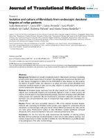
The distribution of the adjusted lung cancer SMR pro-
duced by Analysis 1 (see Table 1 for definition) is
shown in Figure 1. The MCMC random walk generated
a wide spread of posterior SMR ( adjusted SMR) values
with half of the estimates below the reference point of 1.
An overview of the results from all four analyses is
given in Table 2.
Analysis 2 resulted in almost exactly the same findings
from Analysis 1. Very similar results were produced also
by Analyses 3 and 4. Therefore, it made no relevant dif-
ference whether the bias adjustment was based on
Figure 1 Distribution of the posterior lung cancer SMR based an Analysis 1 (see Table 1): previous exposures estimated by the CAREX
method, smoking estimates based on cohort data. Results from an MCMC random walk of length 1,000,000 (Metropolis sampler). The x-axis

stretches to the maximum of 10.7. Other characteristics of this empirical posterior distribution are given in Table 2.
Table 2 Characteristic statistics of the posterior lung cancer SMR distribution, i.e., the distribution of the bias adjusted
SMR.
Analysis
CAREX Expert
smoking cohort smoking case-control smoking cohort smoking case-control
1234
SMR, posterior
median 1.00 1.01 1.32 1.32
arithmetic mean 1.21 1.22 1.33 1.34
standard deviation 0.82 0.83 0.34 0.35
2.5%-fractile 0.24 0.25 0.70 0.70
97.5%-fractile 3.31 3.37 2.04 2.07
Findings are reported according to the four analyses described in Table 1.
The number of significant digits displayed is for comparison purposes only. The data set is not of sufficient size to support this accuracy.
Results from MCMC random walks (Metropolis sampler) of length 1,000,000.
Morfeld and McCunney Journal of Occupational Medicine and Toxicology 2010, 5:23
/>Page 7 of 14
smoking data from the cohort (Analyses 1 and 3) or on
the information gained from the nested case-control
study (Analyses 2 and 4). [This similarity of findings is
somewhat expected because the competing analyses
involve inflating the prior variance of the proportion of
smokers in the cohort This should not affect results
substantially because it is the prior me an of the bias
parameters that dictates the magnitude of unmeasured
confounding.] Lower posterior SMRs were calculated
when using the automatic previous exposure assessment
by the CAREX approach (Analysis 1 an d 2): median
adjusted SMRs were found a t 1, arithme tic averages at

about 1.2. The posterior lung cancer SMR estimates
showed a median and mean of about 1.3 when using
expert data. The analysis based on the CAREX data pro-
duced a wider range of bias adjusted estimates (95%
posterior interval: 0.2, 3.4) than the findings from the
Bayesian analyses when applying the expert’s assessment
(95% posterior interval: 0.7, 2.1).
We performed two additional analyses with the expert’s
data applying a larger spread to the prior distribution of
crystalline silica exposure in the population. Firstly, we
assumed logit
prev, pop
~ N(-5.30, 0.8211) which corre-
sponds to the expert’s prio r as before but with an uncer-
tainty factor of five instead of two. The posterior SMR
was estimated at 1.32 with a 95% posterior interval span-
ning from 0.7 to 2.0. Secondly, we used a prior with an
expectation equal to the CAREX prior but accompanied
with a larger spread ( again corresponding to a factor of
5): logit
prev, pop
~ N(-3.74, 0.8211). In this case, the pos-
terior SMR based on expert data was estimated as 1.40,
95% posterior interval = 0.8, 2.1.
In these analyses we always used a flat prior f or the
SMR. We explored the r obustnessofthisapproachby
applying more concentrated SMR priors. Following [9],
p. 334, 336 we used alternate prior distributions for the
SMR with 95% prior intervals spanning from 0.1 to 10
(corresponding to s = log(10)/1.96 = 1.175 for log SMR)

and 0.25 to 4 (corresponding to s = log(4)/1.96 = 0.707).
The standard deviations are clearly smaller than 10,000
we used in the main analyses. Based on the automatic
approach (CAREX, Analys is 1) we estimated 95% poster-
ior intervals spanning from 0.3 to 3.0 (s = 1.175) and 0.4
to 2.6 (s = 0.707), Analyses applying the expert data
(Analysis 3) returned 95% posterior intervals of 0.7 to 2.0
( s =1.175ands = 0.707), as expected, the medians of
the posterior distributions remained unchanged, i.e., they
were identical to those returned by the main analyses.
Additionally we explored whether a differe nt specifica-
tion of the relative lung cancerriskofsmokers/ex-smo-
kers may affect the results considerably. We averaged
(geometric mean) esti mates for men (active and ex-smo-
kers) from the Nationwide American Cancer Society pro-
spective cohort study ([37], Table Three, full models for
lung cancer) and used RR = 13.3 with 0.95-confidence
limits at 11.0 and 16.0. Applying the alternate prior dis-
tribution for the SMR with 95% prior intervals spanning
from 0.25 to 4 again, the analyses based o n the smoking
effect estimates of Thun et al. 2000 [37] returned a med-
ian posterior SMR of 1.0 with a 95% posterior interval
spanning from 0.4 to 2.5 (CAREX, Analysis 1) and 1.3
(0.7, 1.9) when using expert data (Analysis 3).
Furthermore, we rerun these analyses while incorpor-
ating positive correlations between the draws of smok-
ing prevalences among cohort and population and
between the draws of silica exposure prevalences among
cohort and population. It may be argued that one
expects a higher prevalence among the cohort if the pre-

valence is higher in the population ([9], p. 371, 372). We
implemented these dependencies by applying formula
19-20 in [9], p. 372, and set both correlations between
the logits of prevalences to 0.8 (cp. [9], p. 374). The
modified Analysis 1 (CAREX) returned a median poster-
ior SMR of 1.0 with 95% posterior intervals spanning
from 0.4 to 2.6. The results were 1.3 (0.7, 1.9) when rea-
nalysing the expert data (Analysis 3).
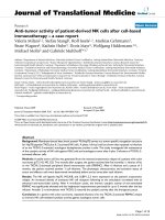
As simple diagnostic tools informing about goodness of
sampler convergence we give trace plots for, e.g., the esti-
mated log SMR (= beta) and the estimated logit of pro-
portion of current or former smokers among unexposed
to carbon black (= xsm_nexp) in Analysis 1 (Figure 2)
and the logit of proportion of current or for mer smokers
among exposed to carbon black (= xsm_exp) and the
logit of proportion of previously exposed to crystalline
silica among exposed to carbon black (= xpq_exp) in
Analysis 4 (Figure 3). The names correspond to variable
names as used in the R program doing the analysis (see
Additional File 3). All the other estimated parameters in
all four analyses showed a similar behaviour as in the
examples presented in Figures 2 and 3.
Discussion
We applied a Bayesian methodology in a cohort study of
German carbon black production workers [6] to adjust
the elevated lung cancer SMR of 2.18 (0.95-CI: 1.61,
2.87) for potential confounding. A nested case-control
study had identified smoking and prev ious occupational
exposures to lung carcinogens received previous to work
at the carbon black plant as potential confounders [8].

We used a Markov Chain Monte Carlo approach
(Metropol is sampler) to quantify the effect of the poten-
tial confounders on the SMR by calculating the distribu-
tion of the posterior SMR[32,33].
The realized acceptance rates between 20% and 40%
were well in the range of published recommendations
[31] and trace plots revealed no problems with the con-
vergence behaviour of the MCMC sampler. Thus, t he
chosen tuning parameters and sampler length of
Morfeld and McCunney Journal of Occupational Medicine and Toxicology 2010, 5:23
/>Page 8 of 14
1,000,000 appear to be appropriate together with a
burn-in phase of 50,000 cycles. Even such long Markov
chains could be realized and evaluated with the R pack-
age [36] on usual laptops or PCs with run times of only
a few minutes (programming code in Additional File 3).
The Bayesian analysis returned a median posterior
SMR estimate in the range between 1.32 (central 0.95-
region: 0.7, 2.1) and 1.00 (c entral 0.95-region: 0.2, 3.3)
depending on how previous exposures were assessed.
The first result is based on an independent expert
assessment of previous exposures combined with a con-
servative a djustment for smoking [5]. The second find-
ing is based on an automatic a pproach (CAREX)
[29,30]. The usually calculated lung cancer SMR statistic
overestimated effect and precision when compared with
the results from the Bayesi an appro ach. This is particu-
larly true when the automatic approach (CAREX)
[29,30] was chosen to assess previous exposures. The
difference in point estimates between both approaches

resulted, at least in part, from the conservative handling
of the smoking adjustment within the fir st approach.
Additional analyses showed that the results based on the
expert’s assessments of prior silica dust exposure among
the carbon black workers changed only slightly when
the prior of the silica dust exposure distribution in the
population was varied.
The CAREX system [29,30] was applied to derive esti-
mates f or crystall ine silica exposure. Obviously, CAREX
may give distorted estimates when a pplied to a specific
group of workers [30]. Although the estimated level of
exposure may be distorted, there is no reason to suspect
a differential misclassification between cases and con-
trols stemming from the same cohort. To validate analy-
tical results ba sed on CAREX estimates w e used
estimates of exposure probabilities generated by an
independent German expert [8]. Agai n, we do not see a
reason to believe in a differential misclassification of
exposures between cases and controls. Because these
approaches are very different we were not surprised get-
ting clearly discrepant estimates of the prevalence of
workers previously exposed to crystalline silica dust in
the carbon black cohort: 74% (CAREX) versus 16%
(expert). However , both very different approaches led to
thesameconclusion:thepreviousexposuretocarcino-
gens received outside the carbon black plant, indicated
by exposure to crystalline silica dust, clearly biased the
Figure 2 Trace plots of log SMR (= beta) and the estimated
logit of proportion of current or former smokers among
unexposed to carbon black (= xsm_nexp). Names (beta,

xsm_nexp) correspond to the variable names used in the R
program (see Additional File 3). Results from an MCMC random
walk of length 1,000,000 (Metropolis sampler) in Analysis 1 (CAREX,
cohort smoking data). Plots include the burn-in phase of 50,000
cycles to give a complete graphical impression of the convergence
behaviour of the Markov chain (Time measures 1,050,000 cycles).
Figure 3 Trace plots of logit of proportion of current or former
smokers among exposed to carbon black (= xsm_exp) and
logit of proportion of previously exposed to crystalline silica
among exposed to carbon black (= xpq_exp). Names (xsm_exp,
xpq_exp) correspond to the variable names used in the R program
(see Additional File 3). Results from an MCMC random walk of
length 1,000,000 (Metropolis sampler) in Analysis 4 (expert’s
assessment, case-control smoking data). Plots include the burn-in
phase of 50,000 cycles to give a complete graphical impression of
the convergence behaviour of the Markov chain (Time measures
1,050,000 cycles).
Morfeld and McCunney Journal of Occupational Medicine and Toxicology 2010, 5:23
/>Page 9 of 14
lung cancer SMR upwards. Thus, both very different
exposure estimation approaches led to similar quantita-
tive corrections of the potentially biased SMR. This con-
sistency is a strength and not a weakness of our
Bayesian bias adjustment procedure.
These findings partially support the results from sim-
ple sensitivity analyses. A corrected lung cancer SMR
was calculated as 1.33 (adjusted 0.95-CI: 0.98, 1.77)
when virtually the same bias adjustments were made
but with the naïve procedures as applied in our earlier
analysis. The derived bias factor depended in the same

degree on smoking and on previous exposures, each
relative bias was estimated to be about 25%. No uncer-
tainties of the bias parameters were taken into account
in that report [5]. As expected, uncertainty was inappro-
priately considered in the simple analysis although the
downward adjusted point estimate correctly conveyed
the large impact of the two biases.
SMR analyses have often been described as prone to
bias [38]. Researcher s have been encouraged to consi der
and quantify the potential distortions or to apply alter-
native analytical procedures. A discussion of these
described limitations of SMR analyses was given by
Morfeld and co-workers [5]. The degree of adjustment
derived in this study may appear surprisingly large in
comparison to discussions of the impact of biases in
occupational epidemiology [39]. However, appropriate
simulation studies showed that a doubling of the relative
risk estimate may easily be produced in realistic epide-
miologic scenarios as a result of residual and unmea-
sured confounding [40].
Crystallinesilicadustexposureisonlyaweaklung
carcinogen [41]. Elevated lung cancer mortalities were
observed [41] at cumulative exposures as high as 6
mg*m
3
-years or even higher [42] and relative risks were
reported to be lower than 1.3 usually. The excess risk
appears to be concentrated on people with silicosis who
showed a doubled lung cancer mortality in comparison
to the general population [43]. However , in our nested

case-control study [8] the variable indicating previous
exposure to crystalline silica dust was found to be signif-
icantly linked to lung cancer mortality with odds ratios
of about 2 or 3 after adjustment for smoking and carbon
black exposure. The lower estimate was based on
CAREX data, the higher one on the expert’s assessment.
Thus, bo th approaches that we applied to estimate pre-
vious exposures to carcinogens resulted in clearly ele-
vated relative risk estimates - although the previous
exposure assessment approaches were independent and
very different in nature. It is important to note that
crystalline silica dust exposure was clearly correlated in
this study with other pre vious exposures to carcinogens,
like a sbestos and PAH exposures. Thus, we interpreted
the crystalline silica dust exposure variable as an
indicator of exposure to a combination of carcinogens
received outside the carbon black plant [8]. We did not
use external relative risk data to adjust for the potential
impact of previous exposures to crystalline silica dust in
this study because partial data on confounders were
available for the cohort of interest. Data describing the
risk situation o f the cohort are usually preferred in
adjustment compared to external data because no addi-
tional exchangeability assumption must be accepted. It
is unusual, for example, to adjust for age in a study by
using population data on lung cancer age trends if an
internal adjustment is possible by the age data of the
cohort at hand. However, an external approach would
be the only way to adjust for confounders if no data on
covariate risk estimation were available for the cohort.

The latter argumentation applies also to smoking sta-
tus as cause of a potential bias in occupational lung can-
cer epidemiology. In this bias analysis we wanted to
exploit the gathered data ab out the workers under study
to the best of our ability. However, it is important to
note that additional external data about the effect of
smok ing (e.g., [37], as applied to a US cohort of crystal-
line silica exposed workers by Steenland and Greenland
[12]) may help to yield narrower posterior intervals -
given that these data are truly applicable to the cohort
under study. A recent overview by the International
Agency for Research on Cancer (IARC) [44] showed a
large variation in lung cancer risk estimates between
investigations (Table 2.1.1.1) and t he IARC working
group compiled evidence for factor s affecting risk like
duration and intensity of smoking, type of cigarette, type
of inhalation, and population characteristics (gender,
ethnicity). The smoking statusvariableasdocumented
in this investigation and other epidemiologic al studies is
only a crude measure and may also code additional life
style and social class differences [45]. Thus it is not easy
to judge whether externally gathered data on the smok-
ing-lung cancer association do really apply - together
with their larger precision. We hesitated to do this in
the main analysis and decided to use only data in this
bias adjustment that was gathered for this cohort and
collected for the embedded case-control study. However,
we applied additio nally relative risk estimates with 0.95-
confdence intervals based on the Nationwide American
Cancer Society prospective coh ort stud y [37] to explore

the impact of the somewhat higher point estimate and
the much smaller confidence interval on the bias correc-
tion. No substantial change in the posterior SMR esti-
mate was observed.
The analyses pres ented suffer from some uncertainties
not quantified. For example, our computations were
based on the assumption that the odds ratios from the
nested case-control study analyses estimated the relative
risks for the co hort in a suitable way and that the
Morfeld and McCunney Journal of Occupational Medicine and Toxicology 2010, 5:23
/>Page 10 of 14
proportion o f subjects with previous occupational expo-
sure to crystalline silica was representative for the
cohort. Such an assumption may hold for the smoking
distribution although based on the sub-cohort with
smoking information only but can be questioned for
cumulative carbon black exposure [8]. Thus, the ques-
tion remains whether the controls were representative
for the previous exposure distribution among the cohort
members. Moreover, some distortions may be due to a
small sample bias [46], an argument relevant for the
analyses based on the expert ass essment of the data. We
applied a conservative correction for smoking, as noted
in an earlier paper, to reduce this potential bias [8].
We applied crude estimates ("guessed factors” )to
quantify the instability of CAREX percentages of occu-
pational crystalline silica exposure in the population and
used an additional adaptation factor to derive population
prevalence estimates for a n analysis applying expert
assessment data. Although these factors could have been

varied in additional sensitivity analyses, we believe that
the uncertainty of these “guesses” is of minor impact on
the results because posterior SMRs showed a wide
spread and the perf ormed sensitivity investigation on
the expert population prior returned no relevant impact
of the varied prior parameter values on the result.
Whether the derived prior distribut ions are indepen-
dent from one another is worthy of discussio n. External
expos ures and tobacco consumption showed some posi-
tive correlation [8], however, correct ion factors for pre-
vious exposures were derived after adjustment for
smoking. We therefore believe that the correction of the
SMR distortion attributed to previous exposures is inde-
pendent of the bias correction due to the differing
smoking b ehaviour in the cohort and the population. A
further assumptio n made is that the confounding biases
are independent of the confounding from measured
variables (like age and calendar time). However, our
ability to specify such correlations knowledgeably is
clearly limited and almost all bias analyses rely on this
assumption (e.g., [12,13,47], see chapter 19 of [9]). How-
ever, implementing correlations of 0.8 between the
draws of the logit of smoking prevalences among cohort
and population and between the draws of the logit of
crystalline s ilica prevalences among cohort and popula-
tion did change the results only negligibly.
A possible distortion due to a healthy worker survivor
bias cannot be ruled out. However, in Cox analyses of
this cohort it was tried to separate out past aspects of
exposure to adjust for survivor biases [7]. Thi s approach

is not fully appropriate. A far better and more valid
adjustment can be performed b y G-estimation [48-51].
However, a considerable amount of detailed longitudinal
data is necessary to generate enough power if that pro-
cedure is applied [52]. Due to the severe power
restriction in this study (only 50 lung cancer deaths
available) an application of Robins’ G-estimation will be
to no avail. Thus, disto rtions due to possi ble survivor
selection effects are not satisfactorily resolved.
We followed Steenland and Greenland [12] and applied
like de Vocht and co-workers [13] an uninformative prior
for the SMR. Strictly speaking, such priors are strange
because extremely high and extremely low relative risks
aregiventhesameprobabilityasrelativerisksina“no r-
mal” range between 0.25 and 4 [18,53]. Thus, it is indi-
cated to apply an informative prior that is more realistic
[9,54]. However, the prior should be “broad enough to
assign relatively high probability to each discussant’s opi-
nion” [15]. A possible occupational cancer risk due to
carbon black exposure is indicated by the occurrence of
lung cancer in rats after inhalation or instillation of car-
bon black and, thus, a working group at the International
Agency for Research on Cancer concluded that there is
sufficien t evidence in experimental animals for the car ci-
nogenicity of carbon black and carbon black extracts [4].
However, Valberg and co-workers [55] summarized their
overview on the carcinogenicity of carbon black as fol-
lows: “new epidemiological evidence decreases concern s
for cancer risks compared with the pre-1996 evidence.
Laboratory studies support a conclusion that the

mechanism of tumorigenicity of CB [carbon black] in
rats is no different from that of any poor ly soluble parti-
cles, ie, toxicity results from the particle overload per se,
and not from the particles’ chemistry”. A leading working
group in particle toxicology concluded [56] that the
observed carcinogenic effect of carbon black is only spe-
cific for rats and that the effects cannot be demonstrated
in mice or hamsters. Moreover, they proposed a thresh-
old effect in rats implying that no canc er hazard exists in
rats (and humans) if exposures are controlled accord-
ingly. This judgement of a limited relevance of the posi-
tive rat experiments with poorly soluble particles is in
line with the consensus report of an expert workshop
held at the ILSI institute [57]. Thus, we think it appropri-
ate to apply a flat prior to the SMR in this analysis cover-
ing without doubt all these opinions about the potential
carcinogenicity of carbon black. Like Steenland and
Greenland [12] we do not think that is a major drawback
to include absurd large and small priors also. The applied
flat SMR prior distribution may help to convince scien-
tists from other faculties not acquainted with Bayesian
thinking that such a bias analysis is a worthwhile exercise
- or even may convi nce freq uentists who resist to a non-
flat prior distribution of the target parameter [58].
However, we explored the robustness of o ur findings
by applying more con centrated SMR priors. Al ternate
prior distributions for the SMR with 95% prior intervals
spanning from 0.1 to 1 0 and 0.25 to 4 produced some-
what narrower interval estimates. The main effect was a
Morfeld and McCunney Journal of Occupational Medicine and Toxicology 2010, 5:23

/>Page 11 of 14
lowering of the upper limits in the CAREX based ana-
lyses. These results did not indicate that t he main an a-
lyses based on flat priors for the SMR were misleading.
Our finding that the elevated lung ca ncer SMR in the
German study cannot be taken as proof for a causal
impact of carbon black exposure on lung c ancer risk is
consistent with the recent decision of an IARC working
group to classify carbon black - based on positive find-
ings in rat experiments - as Group 2B ("possibly carci-
nogenic”) but not as a human lung carcinogen [4]. The
working group stated that “there is inadequate evidence
in humans for the carcinogenicity of carbon black” [4].
Further support of this decision was given by an
updated analysis of two large case-con trol studies in
Montreal: “Subjects with occupational exposure to car-
bon black did not experience any detectable excess
risk of lung cancer” [59].
Bayesian bias analyses - and to a lesser extent, as an
approximation, Monte Carlo sensitivity analyses - are
recommended for combining background data about
biases from different sources [12] p.385, [60] p.47, [9]
p.378-380. In contrast to Monte Carlo Sensitivity Ana-
lyses t he Bayesian method follows a clear mathematical
and philosophical rationale [10], [60] p.53; chapter 18 of
[9], [17]. The Bayesian approach can take into account
correlations between multiple bias estimates and their
different precisions [11]. Even crude estimates of the
probable degree of distortion can be included. This
method is especially valuable when observational studies

are performed with a large number of subjects (high
precision) to quantify small effects sizes (low risk) as
often in genetic or environmental epidemiology [61].
Bayesian analyses may also help to cope with inflated
associations [61]. Overstated effect estimates are to be
expected even if the study is unbiased in the usual sense
[62]. Other authors have also noted the value of Baye-
sian analyses, e.g., to reduce false positives in epidemiol-
ogy [63]. Bayesian false discov ery probability is also
currently used in the analysis of lar ge geneti c data bases
where the danger is rather large that conventional analy-
tical analyses label spurious associations as noteworthy
[64]. Another important application is smoothing by
hierarchical Bayesian models [65]. Markov Chain Monte
Carlo Methods (MCMC) can be used in these analyses
and to perform a Bayesian bias correction, the obje ctive
of this paper, in simple and complicated scenarios [31].
Programming can be done with standard software
packages like the R program [36]. Other recent applica-
tions of Bayesian methods for correcting unmeasured
confounding [13] and misclassification [66] in epidemio-
logical studies are promising examples that this analyti-
cal technique may become a common tool in
epidemiology. Thus, Bayesian bias adjustment can
become a valuable adjunct in occupational and
environmental epidemiology to overcome narrative dis-
cussions of potential distortions.
Conclusions
Bayesian bias adjustment is an excellent tool to quanti-
tatively combine data about confounders f rom different

sources. Markov Chain Monte Carlo Methods (MCMC)
can be used to evaluate Bayes’ theorem even in compli-
cated scenarios. Programming can be done with stan-
dard software like R that is readily available on the web.
Thus, Bayesian bias adjustment can become a regular
tool in occupational and environmental epidem iology to
overcome narrative discussions of potential distortions.
We studied a statistically elevated lung cancer SMR of
2.18 (0.95-CI: 1.61, 2.87) in a German carbon black pro-
duction worker cohort with Bayesian techniques. No link
with carbon black exposure in internal analyses was
noted; potential confounders such as smoking and pre-
vious occupational exposures to carcinogens identified by
a nested case-control study showed that the normally cal-
culated lung cancer SMR overestimated effect and preci-
sion when compared with the MCMC results [median
posterior SMR estimate in the range between 1.32 (cen-
tral 0.95-region: 0.7, 2.1) and 1.00 (central 0.95-region:
0.2, 3.3) depending on the method how previous expo-
sures were assessed]. This finding is consistent with the
conclusion of an IARC working group in 2006 not to
classify carbon black as a human lung carcinogen.
Additional material
Additional file 1: Glossary of key terms. Key terms of the Bayesian
analysis and its implementation are explained.
Additional file 2: Derivation of the bias factor. The bias factor
equation is explained in detail which is applied throughout in the
analyses.
Additional file 3: R program code. R program for Bayesian bias
adjustment of a potentially distorted SMR via Markov Chain Monte Carlo

simulation (Metropolis sampler).
Acknowledgements
The Scientific Advisory Group of the International Carbon Black Association
(ICBA) gave helpful comments on an earlier version of this manuscript. We
would like to thank the reviewers for their critical comments that helped
improve the paper.
Author details
1
Institute for Occupational Medicine of Cologne University/Germany.
2
Institute for Occupational Epidemiology and Risk Assessment of Evonik
Industries, Essen/Germany.
3
Department of Biological Engeneering,
Massachusetts Institute of Technology, Boston/USA.
Authors’ contributions
PM developed the methodology, programmed the code and performed the
analysis. RJM discussed the occupational background (carbon black
production and exposures). Both authors read and approved the final
manuscript.
Morfeld and McCunney Journal of Occupational Medicine and Toxicology 2010, 5:23
/>Page 12 of 14
Competing interests
This study was supported by a grant from the International Carbon Black
Association (ICBA). Both authors serve as Scientific Advisors to this
Association. However, the author s declare that they do not have a conflict
of interest. The ICBA is a scientific, non-profit
corporation originally founded in 1977. The purpose of the ICBA is to
sponsor, conduct, and partic ipate in investigations, research, and analyses
relating to the health, safety, and environmental aspects of the production

and use of carbon black. The manuscript was neither influenced by the ICBA
nor by any company funding the ICBA nor does it present any view or
opinion of the ICBA or of the companies.
Received: 7 June 2010 Accepted: 11 August 2010
Published: 11 August 2010
References
1. International Agency for Research on Cancer: Printing processes and
printing inks, carbon black and some nitro compounds. IARC
monographs on the evaluation of carcinogenic risks to humans Lyon: IARC
1996, 65:1-578.
2. Wang M-J, Nissen MH, Buus S, Röpke C, Claësson MH: Comparison of CTL
reactivity in the spleen and draining lymph nodes after immunization
with peptides pulsed on dendritic cells or mixed with Freund’s
incomplete adjuvant. Immunology Letters 2003, 90:13-18.
3. McCunney RJ, Muranko HJ, Valberg PA: Carbon black. Patty’s Toxicology
New York: John Wiley & SonsBingham E, Cohrssen B, Powell CH , Fifth 2001,
8:1081-1101.
4. Baan RA: Carcinogenic hazards from inhaled carbon black, titanium
dioxide, and talc not containing asbestos or asbestiform fibers: recent
evaluations by an IARC Monographs Working Group. Inhal Toxicol 2007,
19(Suppl 1):213-228.
5. Morfeld P, Büchte SF, McCunney RJ, Piekarski C: Lung cancer mortality and
carbon black exposure: uncertainties of SMR analyses in a cohort study
at a German carbon black production plant. J Occup Environ Med 2006,
48:1253-1264.
6. Wellmann J, Weiland SK, Neiteler G, Klein G, Straif K: Cancer mortality in
German carbon black workers 1976-1998. Occup Environ Med 2006,
63:513-521.
7. Morfeld P, Büchte SF, Wellmann J, McCunney RJ, Piekarski C: Lung cancer
mortality and carbon black exposure: cox regression analysis of a cohort

from a German carbon black production plant. J Occup Environ Med 2006,
48:1230-1241.
8. Büchte SF, Morfeld P, Wellmann J, Bolm-Audorff U, McCunney RJ,
Piekarski C: Lung cancer mortality and carbon black exposure: a nested
case-control study at a German carbon black production plant. J Occup
Environ Med 2006, 48:1242-1252.
9. Rothman KJ, Greenland S, Lash TL: Modern epidemiology Philadelphia:
Lippincott Williams & Wilkins, 3 2008.
10. Greenland S: Sensitivity analysis, Monte Carlo risk analysis, and Bayesian
uncertainty assessment. Risk Anal 2001, 21:579-583.
11. Greenland S: Bayesian perspectives for epidemiologic research: III. Bias
analysis via missing-data methods. Int J Epidemiol 2009, 38:1662-1673.
12. Steenland K, Greenland S: Monte Carlo sensitivity analysis and Bayesian
analysis of smoking as an unmeasured confounder in a study of silica
and lung cancer. Am J Epidemiol 2004, 160:384-392.
13. de Vocht F, Kromhout H, Ferro G, Boffetta P, Burstyn I: Bayesian modeling
of lung cancer risk and bitumen fume exposure adjusted for
unmeasured confounding by smoking. Occup Environ Med 2008, 22.
14. Lee PM: Bayesian statistics: an introduction London: Arnold, 2 2003.
15. Greenland S: Bayesian perspectives for epidemiological research: I.
Foundations and basic methods. Int J Epidemiol 2006, 35:765-775.
16. Greenland S: Bayesian perspectives for epidemiological research. II.
Regression analysis. Int J Epidemiol 2007, 36:195-202.
17. Lindley DV: The philosophy of statistics. The Statistician 2000, 49(Part
3):293-337.
18. Greenland S: Probability logic and probabilistic induction. Epidemiol 1998,
9:322-332.
19. Breslow NE, Day NE: Statistical methods in cancer research. Volume II-The
design and analysis of cohort studies Lyon: International Agency for Research
on Cancer 1987.

20. Maldonado G: Adjusting a relative-risk estimate for study imperfections. J
Epidemiol Community Health 2008, 62:655-663.
21. Cornfield J, Haenszel W, Hammond EC, Lilienfeld AM, Shimkin MB,
Wynder EL: Smoking and lung cancer: recent evidence and a discussion
of some questions. J Natl Cancer Inst 1959, 22:173-203.
22. Cornfield J, Haenszel W, Hammond EC, Lilienfeld AM, Shimkin MB,
Wynder EL: Smoking and lung cancer: recent evidence and a discussion
of some questions. 1959. Int J Epidemiol 2009, 38:1175-1191.
23. Bross ID: Spurious effects from an extraneous variable. J Chronic Dis 1966,
19:637-647.
24. Yanagawa T: Case-control studies: assessing the effect of a confounding
factor. Biometrika 1984, 71:191-194.
25. Axelson O, Steenland K: Indirect methods of assessing the effects of
tobacco use in occupational studies. Am J Ind Med 1988, 13:105-118.
26. Rothman KJ, Greenland S: Modern epidemiology Philadelphia: Lippincott -
Raven, 2 1998.
27. Junge B, Nagel M: Das Rauchverhalten in Deutschland. Gesundheitswesen
1999, 61(Sonderheft 2):121-125.
28. Thefeld W, Stolzenberg H, Bellach B-M: Bundes-Gesundheitssurvey:
Response, Zusammensetzung der Teilnehmer und Non-Responder-
Analyse. Gesundheitswesen 1999, 61(Sonderheft 2):S57-S61.
29. CAREX: 2005 [ />30. Kauppinen T, Toikkanen J, Pedersen D, Young R, Ahrens W, Boffetta P,
Hansen J, Kromhout H, Maqueda Blasco J, Mirabelli D, et al: Occupational
exposure to carcinogens in the European Union. Occup Environ Med
2000, 57:10-18.
31. Gilks WR, Richardson S, Spiegelhalter DJ, (Eds):
Markov chain Monte Carlo in
practice Coca Raton: Chapman & HALL/CRC 1996.
32. Metropolis N, Rosenbluth AW, Rosenbluth MN, Teller AH, Teller E: Equations
of state calculations by fast computing machines. J Chem Phys 1953,

21:1087-1092.
33. Hastings WK: Monte Carlo sampling methods using Markow chains and
their applications. Biometrika 1970, 57:97-109.
34. Newman K: Bayesian inference (Lecture Notes) University of St. Andrews 2005
[ />35. SAS/STAT(R) 9.2: User’s Guide, Second Edition: Introduction to Bayesian
Analysis Procedures: Assessing Markov Chain Convergence 2009 [http://
support.sas.com/documentation/cdl/en/statug/63033/HTML/default/
statug_introbayes_sect008.htm].
36. R Development Core Team: R: A Language and environment for
statistical computing. Vienna, Austria Foundation for statistical computing
2008 [].
37. Thun MJ, Apicella LF, Henley SJ: Smoking vs other risk factors as the
cause of smoking-attributable deaths: confounding in the courtroom.
JAMA 2000, 284:706-712.
38. Park RM, Maizlish NA, Punnett L, Moure-Eraso R, Silverstein MA: A
comparison of PMRs and SMRs as estimators of occupational mortality.
Epidemiol 1991, 2:49-59.
39. Blair A, Stewart P, Lubin JH, Forastiere F: Methodological issues regarding
confounding and exposure misclassification in epidemiological studies
of occupational exposures. Am J Ind Med 2007, 50:199-207.
40. Fewell Z, Davey Smith G, Sterne JA: The impact of residual and
unmeasured confounding in epidemiologic studies: a simulation study.
Am J Epidemiol 2007, 166:646-655.
41. Steenland K, Mannetje A, Boffetta P, Stayner L, Attfield M, Chen J,
Dosemeci M, DeKlerk N, Hnizdo E, Koskela R, Checkoway H: Pooled
exposure-response analyses and risk assessment for lung cancer in 10
cohorts of silica-exposed workers: an IARC multicentre study. Cancer
Causes Control 2001, 12:773-784, Erratum in:Cancer Causes 2013:2777.
42. Pukkala E, Guo J, Kyyronen P, Lindbohm M-L, Sallmen M, Kauppinen T:
National job-exposure matrix in analyses of census-based estimates of

occupational cancer risk. Scand J Work Environ Health 2005, 31:97-107.
43. Erren TC, Glende CB, Morfeld P, Piekarski C: Is exposure to silica associated
with lung cancer in the absence of silicosis? A meta-analytical approach
to an important public health question. Int Arch Occup Environ Health
2008, 8.
44. IARC: Tobacco smoke and involuntary smoking Lyon: International Agency
for Research on Cancer 2004.
45. Soutar CA, Robertson A, Miller BG, Searl A, Bignon J: Epidemiological
evidence on the carcinogenicity of silica: factors in scientific judgement.
Ann Occup Hyg 2000, 44:3-14.
Morfeld and McCunney Journal of Occupational Medicine and Toxicology 2010, 5:23
/>Page 13 of 14
46. Greenland S, Schwartzbaum JA, Finkle WD: Problems due to small
samples and sparse data in conditional logistic regression analysis. Am J
Epidemiol 2000, 151:531-539.
47. McCandless LC, Gustafson P, Levy A: Bayesian sensitivity analysis for
unmeasured confounding in observational studies. Stat Med 2007,
26:2331-2347.
48. Morfeld P: Years of life lost due to exposure: causal concepts and
empirical shortcomings. Epidemiol Perspect Innov 2004 [-
perspectives.com/content/1/1/5].
49. Witteman JCM, D’Agostino RB, Stijnen T, Kannel WB, Cobb JC, de
Ridder MA, Hofman A, Robins JM: G-estimation of causal effects: isolated
systolic hypertension and cardiovascular death in the Framingham Heart
Study. Am J Epidemiol 1998, 148:390-401.
50. Robins JM: Causal inference from complex longitudinal data. Latent
variable modeling with applications to causality New York: Springer-
VerlagBerkane M 1997, 69-117.
51. Robins JM, Greenland S: Adjusting for differential rates of prophylayis
therapy for PCP in high- versus low-dose AZT treatment arms in an

AIDS randomized trial. J Am Statist Ass 1994, 89:737-749.
52. Morfeld P, Lampert K, Emmerich M, Stegmaier C, Piekarski C: Adjusting for
dependent censoring, survivor biases and confounders: a cohort study
on lung cancer risk in German coalminers. 16
th
International Symposium
Epidemiology. Med Lav 2002, 93:373.
53. Greenland S: Putting background information about relative risks into
conjugate prior distributions. Biometrics 2001, 57:663-670.
54. Thomas DC, Jerrett M, Kuenzli N, Louis TA, Dominici F, Zeger S, Schwarz J,
Burnett RT, Krewski D, Bates D: Bayesian model averaging in time-series
studies of air pollution and mortality. J Toxicol Environ Health A 2007,
70:311-315.
55. Valberg PA, Long CM, Sax SN: Integrating studies on carcinogenic risk of
carbon black: epidemiology, animal exposures, and mechanism of
action. J Occup Environ Med 2006, 48:1291-1307.
56. Carter JM, Corson N, Driscoll KE, Elder A, Finkelstein JN, Harkema JN,
Gelein R, Wade-Mercer P, Nguyen K, Oberdorster G: A comparative dose-
related response of several key pro- and antiinflammatory mediators in
the lungs of rats, mice, and hamsters after subchronic inhalation of
carbon black. J Occup Environ Med 2006, 48:1265-1278.
57. ILSI: The relevance of the rat lung response to particle overload for
human risk assessment: A workshop consensus report - Risk Science
Institute Workshop. Inhal Toxicol 2000, 12:1-17.
58. Lash TL: Heuristic thinking and inference from observational
epidemiology. Epidemiol 2007, 18:67-72.
59. Ramanakumar AV, Parent M-É, Latreille B, Siemiatycki J: Risk of lung cancer
following exposure to carbon black, titanium dioxide and talc: results
from two case-control studies in Montreal. Int J Cancer 2008, 122:183-189.
60. Greenland S: The impact of prior distributions of uncontrolled

confounding and response bias: a case study of the relation of wire
codes and magnetic fields to childhood leukemia. J Am Stat Assoc 2003,
98:47-54.
61. Ioannidis JPA: Why most discovered true associations are inflated.
Epidemiol 2008, 19:640-648.
62. Senn S: Transposed conditionals, shrinkage, and direct and indirect
unbiasedness. Epidemiol 2008, 19:652-654, discussion 657-658.
63. Boffetta P, McLaughlin JK, La Vecchia C, Tarone RE, Lipworth L, Blot WJ:
False-positive results in cancer epidemiology: a plea for epistemological
modesty. J Natl Cancer Inst 2008, 100:988-995.
64. Wakefield J: A Bayesian measure of the probability of false discovery in
genetic epidemiology studies. Am J Hum Genet 2007, 81:208-227.
65. Graham P: Intelligent smoothing using hierarchical Bayesian models.
Epidemiol 2008, 19:493-495.
66. MacLehose RF, Olshan AF, Herring AH, Honein MA, Shaw GM, Romitti PA:
Bayesian methods for correcting misclassification. An example from
birth defects epidemiology. Epidemiol
2009, 20:27-35.
doi:10.1186/1745-6673-5-23
Cite this article as: Morfeld and McCunney: Bayesian bias adjustments
of the lung cancer SMR in a cohort of German carbon black production
workers. Journal of Occupational Medicine and Toxicology 2010 5:23.
Submit your next manuscript to BioMed Central
and take full advantage of:
• Convenient online submission
• Thorough peer review
• No space constraints or color figure charges
• Immediate publication on acceptance
• Inclusion in PubMed, CAS, Scopus and Google Scholar
• Research which is freely available for redistribution

Submit your manuscript at
www.biomedcentral.com/submit
Morfeld and McCunney Journal of Occupational Medicine and Toxicology 2010, 5:23
/>Page 14 of 14