matlab recipes for earth sciences - m.h.trauth
Bạn đang xem bản rút gọn của tài liệu. Xem và tải ngay bản đầy đủ của tài liệu tại đây (4.37 MB, 240 trang )
Martin H. Trauth
MATLAB
®
Recipes for Earth Sciences
Martin H. Trauth
MATLAB
®
Recipes
for Earth Sciences
With text contributions by
Robin Gebbers and Norbert Marwan
and illustrations by Elisabeth Sillmann
With 77 Figures and a CD-ROM
Privatdozent Dr. rer. nat. habil.
M.H. Trauth
University of Potsdam
Department of Geosciences
P.O. Box 60 15 53
14415 Potsdam
Germany
E-mail:
Copyright disclaimer
MATLAB
®
is a trademark of The MathWorks, Inc. and is used with permission. The MathWorks
does not warrant the accuracy of the text or exercises in this book. This book’s use or discussion of
MATLAB
®
software or related products does not constitute endorsement or sponsorship by The
MathWorks of a particular pedagogical approach or particular use of the MATLAB
®
software.
For MATLAB
®
product information, please contact:
The MathWorks, Inc.
3 Apple Hill Drive
Natick, MA, 01760-2098 USA
Tel: 508-647-7000
Fax: 508-647-7001
E-mail:
Web: www.mathworks.com
Library of Congress Control Number: 2005937738
ISBN-10 3-540-27983-0 Springer Berlin Heidelberg New York
ISBN-13 978-3540-27983-9 Springer Berlin Heidelberg New York
This work is subject to copyright. All rights are reserved, whether the whole or part of the
material is concerned, specifically the rights of translation, reprinting, reuse of illustra-
tions, recitation, broadcasting, reproduction on microfilm or in any other way, and stor-
age in data banks. Duplication of this publication or parts thereof is permitted only un-
der the provisions of the German Copyright Law of September 9, 1965, in its current
version, and permission for use must always be obtained from Springer-Verlag. Viola-
tions are liable to prosecution under the German Copyright Law.
Springer is a part of Springer Science+Business Media
Springer.com
© Springer-Verlag Berlin Heidelberg 2006
Printed in The Netherlands
The use of general descriptive names, registered names, trademarks, etc. in this publica-
tion does not imply, even in the absence of a specific statement, that such names are ex-
empt from the relevant protective laws and regulations and therefore free for general use.
Cover design: Erich Kirchner
Typesetting: camera-ready by Elisabeth Sillmann, Landau
Production: Christine Jacobi
Printing: Krips bv, Meppel
Binding: Stürtz AG, Würzburg
Printed on acid-free paper 32/2132/cj 5 4 3 2 1 0
Preface
Various books on data analysis in earth sciences have been published during
the last ten years, such as Statistics and Data Analysis in Geology by JC Davis,
Introduction to Geological Data Analysis by ARH Swan and M Sandilands,
Data Analysis in the Earth Sciences Using MATLAB
®
by GV Middleton or
Statistics of Earth Science Data by G Borradaile. Moreover, a number of
software packages have been designed for earth scientists such as the ESRI
product suite ArcGIS or the freeware package GRASS for generating geo-
graphic information systems, ERDAS IMAGINE or RSINC ENVI for remote
sensing and GOCAD and SURFER for 3D modeling of geologic features. In
addition, more general software packages as IDL by RSINC and MATLAB
®
by The MathWorks Inc. or the freeware software OCTAVE provide powerful
tools for the analysis and visualization of data in earth sciences.
Most books on geological data analysis contain excellent theoreti-
cal introductions, but no computer solutions to typical problems in earth
sciences, such as the book by JC Davis. The book by ARH Swan and
M Sandilands contains a number of examples, but without the use of com-
puters. G Middleton·s book fi rstly introduces MATLAB as a tool for earth
scientists, but the content of the book mainly refl ects the personal interests
of the author, rather then providing a complete introduction to geological
data analysis. On the software side, earth scientists often encounter the prob-
lem that a certain piece of software is designed to solve a particular geologic
problem, such as the design of a geoinformation system or the 3D visualiza-
tion of a fault scarp. Therefore, earth scientists have to buy a large volume
of software products, and even more important, they have to get used to it
before being in the position to successfully use it.
This book on MATLAB Recipes for Earth Sciences is designed to help
undergraduate and PhD students, postdocs and professionals to learn meth-
ods of data analysis in earth sciences and to get familiar with MATLAB,
the leading software for numerical computations. The title of the book is
an appreciation of the book Numerical Recipes by WH Press and others
that is still very popular after initially being published in 1986. Similar to
the book by Press and others, this book provides a minimum amount of
VI Preface
theoretical background, but then tries to teach the application of all methods
by means of examples. The software MATLAB is used since it provides
numerous ready-to-use algorithms for most methods of data analysis, but
also gives the opportunity to modify and expand the existing routines and
even develop new software. The book contains numerous MATLAB scripts
to solve typical problems in earth sciences, such as simple statistics, time-
series analysis, geostatistics and image processing. The book comes with a
compact disk, which contains all MATLAB recipes and example data fi les.
All MATLAB codes can be easily modifi ed in order to be applied to the
reader·s data and projects.
Whereas undergraduates participating in a course on data analysis might
go through the entire book, the more experienced reader will use only one
particular method to solve a specifi c problem. To facilitate the use of this
book for the various readers, I outline the concept of the book and the con-
tents of its chapters.
1. Chapter 1 – This chapter introduces some fundamental concepts of sam-
ples and populations, it links the various types of data and questions to
be answered from these data to the methods described in the following
chapters.
2. Chapter 2 – A tutorial-style introduction to MATLAB designed for earth
scientists. Readers already familiar with the software are advised to pro-
ceed directly to the following chapters.
3. Chapter 3 and 4 – Fundamentals in univariate and bivariate statistics.
These chapters contain very basic things how statistics works, but also
introduce some more advanced topics such as the use of surrogates. The
reader already familiar with basic statistics might skip these two chap-
ters.
4. Chapter 5 and 6 – Readers who wish to work with time series are recom-
mended to read both chapters. Time-series analysis and signal processing
are tightly linked. A solid knowledge of statistics is required to success-
fully work with these methods. However, the two chapters are more or
less independent from the previous chapters.
5. Chapter 7 and 8 – The second pair of chapters. From my experience,
reading both chapters makes a lot of sense. Processing gridded spatial
data and analyzing images has a number of similarities. Moreover, aerial
Preface VII
photographs and satellite images are often projected upon digital eleva-
tion models.
6. Chapter 9 – Data sets in earth sciences are tremendously increasing in the
number of variables and data points. Multivariate methods are applied to
a great variety of types of large data sets, including even satellite images.
The reader particularly interested in multivariate methods is advised to
read Chapters 3 and 4 before proceeding to this chapter.
I hope that the various readers will now fi nd their way through the book.
Experienced MATLAB users familiar with basic statistics are invited to pro-
ceed to Chapters 5 and 6 (the time series), Chapters 7 and 8 (spatial data and
images) or Chapter 9 (multivariate analysis) immediately, which contain
both an introduction to the subjects as well as very advanced and special
procedures for analyzing data in earth sciences. It is recommended to the
beginners, however, to read Chapters 1 to 4 carefully before getting into the
advanced methods.
I thank the NASA/GSFC/METI/ERSDAC/JAROS and U.S./Japan ASTER
Science Team and the director Mike Abrams for allowing me to include the
ASTER images in the book. The book has benefi t from the comments of a
large number of colleagues and students. I gratefully acknowledge my col-
leagues who commented earlier versions of the manuscript, namely Robin
Gebbers, Norbert Marwan, Ira Ojala, Lydia Olaka, Jim Renwick, Jochen
Rössler, Rolf Romer, and Annette Witt. Thanks also to the students Mathis
Hein, Stefanie von Lonski and Matthias Gerber, who helped me to improve
the book. I very much appreciate the expertise and patience of Elisabeth
Sillmann who created the graphics and the complete page design of the
book. I also acknowledge Courtney Esposito leading the author program at
The MathWorks, Claudia Olrogge and Annegret Schumann at Mathworks
Deutschland, Wolfgang Engel at Springer, Andreas Bohlen and Brunhilde
Schulz at UP Transfer GmbH. I would like to thank Thomas Schulmeister
who helped me to get a campus license for MATLAB at Potsdam University.
The book is dedicated to Peter Koch, the late system administrator of the
Department of Geosciences who died during the fi nal writing stages of the
manuscript and who helped me in all kinds of computer problems during the
last few years.
Potsdam, September 2005
Martin Trauth
Contents
Preface V
1 Data Analysis in Earth Sciences 1
1.1 Introduction 1
1.2 Collecting Data 1
1.3 Types of Data 3
1.4 Methods of Data Analysis 7
2 Introduction to MATLAB 11
2.1 MATLAB in Earth Sciences 11
2.2 Getting Started 12
2.3 The Syntax 15
2.4 Data Storage 19
2.5 Data Handling 19
2.6 Scripts and Functions 21
2.7 Basic Visualization Tools 25
3 Univariate Statistics 29
3.1 Introduction 29
3.2 Empirical Distributions 29
3.3 Example of Empirical Distributions 36
3.4 Theoretical Distributions 41
3.5 Example of Theoretical Distributions 50
3.6 The t–Test 51
3.7 The F–Test 53
3.8 The
χ
2
–Test 56
X Contents
4 Bivariate Statistics 61
4.1 Introduction 61
4.2 Pearson·s Correlation Coeffi cient 61
4.3 Classical Linear Regression Analysis and Prediction 68
4.5 Analyzing the Residuals 72
4.6 Bootstrap Estimates of the Regression Coeffi cients 74
4.7 Jackknife Estimates of the Regression Coeffi cients 76
4.8 Cross Validation 77
4.9 Reduced Major Axis Regression 78
4.10 Curvilinear Regression 80
5 Time-Series Analysis 85
5.1 Introduction 85
5.2 Generating Signals 85
5.3 Autospectral Analysis 91
5.4 Crossspectral Analysis 97
5.5 Interpolating and Analyzing Unevenly-Spaced Data 101
5.6 Nonlinear Time-Series Analysis (by N. Marwan) 106
6 Signal Processing 119
6.1 Introduction 119
6.2 Generating Signals 120
6.3 Linear Time-Invariant Systems 121
6.4 Convolution and Filtering 124
6.5 Comparing Functions for Filtering Data Series 127
6.6 Recursive and Nonrecursive Filters 129
6.7 Impulse Response 131
6.8 Frequency Response 134
6.9 Filter Design 139
6.10 Adaptive Filtering 143
7 Spatial Data 151
7.1 Types of Spatial Data 151
7.2 The GSHHS Shoreline Data Set 152
7.3 The 2-Minute Gridded Global Elevation Data ETOPO2 154
7.4 The 30-Arc Seconds Elevation Model GTOPO30 157
Contents XI
7.5 The Shuttle Radar Topography Mission SRTM 158
7.6 Gridding and Contouring Background 161
7.7 Gridding Example 164
7.8 Comparison of Methods and Potential Artifacts 169
7.9 Geostatistics (by R. Gebbers) 173
8 Image Processing 193
8.1 Introduction 193
8.2 Data Storage 194
8.3 Importing, Processing and Exporting Images 199
8.4 Importing, Processing and Exporting Satellite Images 204
8.5 Georeferencing Satellite Images 207
8.6 Digitizing from the Screen 209
9 Multivariate Statistics 213
9.1 Introduction 213
9.2 Principal Component Analysis 214
9.3 Cluster Analysis 221
9.4 Independent Component Analysis (by N. Marwan) 225
General Index 231
1 Data Analysis in Earth Sciences
1.1 Introduction
Earth sciences include all disciplines that are related to our planet Earth.
Earth scientists make observations and gather data, they formulate and test
hypotheses on the forces that have operated in a certain region in order to
create its structure. They also make predictions about future changes of the
planet. All these steps in exploring the system Earth include the acquisition
and analysis of numerical data. An earth scientist needs a solid knowledge in
statistical and numerical methods to analyze these data, as well as the ability
to use suitable software packages on a computer.
This book introduces some of the most important methods of data analy-
sis in earth sciences by means of MATLAB examples. The examples can
be used as recipes for the analysis of the reader·s real data after learn-
ing their application on synthetic data. The introductory Chapter 1 deals
with data acquisition (Chapter 1.2), the expected data types (Chapter 1.3)
and the suitable methods for analyzing data in the fi eld of earth sciences
(Chapter 1.4). Therefore, we fi rst explore the characteristics of a typical data
set. Subsequently, we proceed to investigate the various ways of analyzing
data with MATLAB.
1.2 Collecting Data
Data sets in earth sciences have a very limited sample size. They also con-
tain a signifi cant amount of uncertainties. Such data sets are typically used
to describe rather large natural phenomena such as a granite body, a large
landslide or a widespread sedimentary unit. The methods described in this
book help in fi nding a way of predicting the characteristics of a larger pop-
ulation from the collected samples (Fig 1.1). In this context, a proper sam-
pling strategy is the fi rst step towards obtaining a good data set. The devel-
opment of a successful strategy for fi eld sampling includes decisions on
2 1 Data Analysis in Earth Sciences
1. the sample size – This parameter includes the sample volume or its weight
as well as the number of samples collected in the fi eld. The rock weight
or volume can be a critical factor if the samples are later analyzed in the
laboratory. On the application of certain analytic techniques a specifi c
amount of material may be required. The sample size also restricts the
number of subsamples that eventually could be collected from the single
sample. If the population is heterogeneous, then the sample needs to be
large enough to represent the population·s variability. On the other hand,
a sample should always be as small as possible in order to save time and
effort to analyze it. It is recommended to collect a smaller pilot sample
before defi ning a suitable sample size.
Fig. 1.1 Samples and population. Deep valley incision has eroded parts of a sandstone unit
(hypothetical population). The remnants of the sandstone ( available population) can only
be sampled from outcrops, i.e., road cuts and quarries ( accessible population). Note the
difference between a statistical sample as a representative of a population and a geological
sample as a piece of rock.
Geological
sample
Accessible
Population
Road cut
Outcrop
River valley
Available
Population
Hypothetical
Population
1.3 Types of Data 3
2. the spatial sampling scheme – In most areas, samples are taken as the
availability of outcrops permits. Sampling in quarries typically leads to
clustered data, whereas road cuts, shoreline cliffs or steep gorges cause
traverse sampling schemes. If money does not matter or the area allows
hundred percent access to the rock body, a more uniform sampling pat-
tern can be designed. A regular sampling scheme results in a gridded dis-
tribution of sample locations, whereas a uniform sampling strategy in-
cludes the random location of a sampling point within a grid square. You
might expect that these sampling schemes represent the superior method
to collect the samples. However, equally-spaced sampling locations tend
to miss small-scale variations in the area, such as thin mafi c dykes in a
granite body or spatially-restricted occurrence of a fossil. In fact, there is
no superior sample scheme, as shown in Figure 1.2.
The proper sampling strategy depends on the type of object to be analyzed,
the purpose of the investigation and the required level of confi dence of the
fi nal result. Having chosen a suitable sampling strategy, a number of distur-
bances can infl uence the quality of the set of samples. The samples might
not be representative of the larger population if it was affected by chemi-
cal or physical alteration, contamination by other material or the sample
was dislocated by natural or anthropogenic processes. It is therefore recom-
mended to test the quality of the sample, the method of data analysis em-
ployed and the validity of the conclusions based on the analysis in all stages
of the investigation.
1.3 Types of Data
These data types are illustrated in Figure 1.3. The majority of the data con-
sist of numerical measurements, although some information in earth sci-
ences can also be represented by a list of names such as fossils and minerals.
The available methods for data analysis may require certain types of data in
earth sciences. These are
1. nominal data – Information in earth sciences is sometimes presented as
a list of names, e.g., the various fossil species collected from a limestone
bed or the minerals identifi ed in a thin section. In some studies, these
data are converted into a binary representation, i.e., one for present and
zero for absent. Special statistical methods are available for the analysis
of such data sets.
4 1 Data Analysis in Earth Sciences
ab
cd
e
First Road
Second Road
Boreholes
First Road
Second Road
Boreholes
First Road
Second Road
First Road
Second Road
Boreholes
Quarry
Samples
First Road
Second Road
Samples
R
i
v
e
r
V
a
l
l
e
y
Samples
Road cuts
Fig. 1.2 Sampling schemes. a Regular sampling on an evenly-spaced rectangular grid,
b uniform sampling by obtaining samples randomly-located within regular grid squares,
c random sampling using uniform-distributed xy coordinates, d clustered sampling
constrained by limited access, and e traverse sampling along road cuts and river valleys.
1.3 Types of Data 5
Cyclotella ocellata
C. meneghiniana
C. ambigua
C. agassizensis
Aulacoseira granulata
A. granulata var. curvata
A. italica
Epithemia zebra
E. sorex
Thalassioseira faurii
1. Talc
2. Gypsum
3. Calcite
4. Flurite
5. Apatite
6. Orthoclase
7. Quartz
8. Topaz
9. Corundum
10. Diamond
01234567
2.5 4.0 7.0
-3-2-101234
-0.5 +2.0 +4.0
0255075
30 50 82.5%
100%
N
31
28
25
27
30
33
N
EW
S
110°
70°
45°
ab
ef
g
cd
EW
S
N
Fig. 1.3 Types of data in earth sciences. a Nominal data, b ordinal data, c ratio data,
d interval data, e closed data, f spatial data and g directional data. For explanation see text.
All data types are described in the book except for directional data since there are better tools
to analyze such data in earth sciences than MATLAB.
6 1 Data Analysis in Earth Sciences
2. ordinal data – These are numerical data representing observations that
can be ranked, but the intervals along the scale are not constant. Mohs·
hardness scale is one example for an ordinal scale. The Mohs· hardness
value indicates the materials resistance to scratching. Diamond has a hard-
ness of 10, whereas this value for talc is 1. In terms of absolute hardness,
diamond (hardness 10) is four times harder than corundum (hardness 9)
and six times harder than topaz (hardness 8). The Modifi ed Mercalli Scale
to categorize the size of earthquakes is another example for an ordinal
scale. It ranks earthquakes from intensity I (barely felt) to XII (total de-
struction).
3. ratio data – The data are characterized by a constant length of successive
intervals. This quality of ratio data offers a great advantage in comparison
to ordinal data. However, the zero point is the natural termination of the
data scale. Examples of such data sets include length or weight data. This
data type allows either a discrete or continuous data sampling.
4. interval data – These are ordered data that have a constant length of suc-
cessive intervals. The data scale is not terminated by zero. Temperatures
C and F represent an example of this data type although zero points exist
for both scales. This data type may be sampled continuously or in discrete
intervals.
Besides these standard data types, earth scientists frequently encounter spe-
cial kinds of data, such as
1. closed data – These data are expressed as proportions and add to a fi xed
total such as 100 percent. Compositional data represent the majority of
closed data, such as element compositions of rock samples.
2. spatial data – These are collected in a 2D or 3D study area. The spatial
distribution of a certain fossil species, the spatial variation of the sand-
stone bed thickness and the 3D tracer concentration in groundwater are
examples for this data type. This is likely to be the most important data
type in earth sciences.
3. directional data – These data are expressed in angles. Examples include
the strike and dip of a bedding, the orientation of elongated fossils or the
fl ow direction of lava. This is a very frequent data type in earth sciences.
1.4 Methods of Data Analysis 7
Most of these data require special methods to be analyzed, that are outlined
in the next chapter.
1.4 Methods of Data Analysis
Data analysis methods are used to describe the sample characteristics as
precisely as possible. Having defi ned the sample characteristics we proceed
to hypothesize about the general phenomenon of interest. The particular
method that is used for describing the data depends on the data type and the
project requirements.
1. Univariate methods – Each variable in a data set is explored separately
assuming that the variables are independent from each other. The data are
presented as a list of numbers representing a series of points on a scaled
line. Univariate statistics includes the collection of information about
the variable, such as the minimum and maximum value, the average and
the dispersion about the average. Examples are the investigation of the
sodium content of volcanic glass shards that were affected by chemical
weathering or the size of fossil snail shells in a sediment layer.
2. Bivariate methods – Two variables are investigated together in order to
detect relationships between these two parameters. For example, the cor-
relation coeffi cient may be calculated in order to investigate whether there
is a linear relationship between two variables. Alternatively, the bivariate
regression analysis may be used to describe a more general relationship
between two variables in the form of an equation. An example for a bi-
variate plot is the Harker Diagram, which is one of the oldest method
to visualize geochemical data and plots oxides of elements against SiO2
from igneous rocks.
3. Time-series analysis – These methods investigate data sequences as a
function of time. The time series is decomposed into a long-term trend,
a systematic (periodic, cyclic, rhythmic) and an irregular (random, sto-
chastic) component. A widely used technique to analyze time series is
spectral analysis, which is used to describe cyclic components of the
time series. Examples for the application of these techniques are the
investigation of cyclic climate variations in sedimentary rocks or the
analysis of seismic data.
8 1 Data Analysis in Earth Sciences
4. Signal processing – This includes all techniques for manipulating a signal
to minimize the effects of noise, to correct all kinds of unwanted distor-
tions or to separate various components of interest. It includes the design,
realization and application of fi lters to the data. These methods are widely
used in combination with time-series analysis, e.g., to increase the signal-
to-noise ratio in climate time series, digital images or geophysical data.
5. Spatial analysis – The analysis of parameters in 2D or 3D space. Therefore,
two or three of the required parameters are coordinate numbers. These
methods include descriptive tools to investigate the spatial pattern of geo-
graphically distributed data. Other techniques involve spatial regression
analysis to detect spatial trends. Finally, 2D and 3D interpolation tech-
niques help to estimate surfaces representing the predicted continuous
distribution of the variable throughout the area. Examples are drainage-
system analysis, the identifi cation of old landscape forms and lineament
analysis in tectonically-active regions.
6. Image processing – The processing and analysis of images has become
increasingly important in earth sciences. These methods include manipu-
lating images to increase the signal-to-noise ratio and to extract certain
components of the image. Examples for this analysis are analyzing satel-
lite images, the identifi cation of objects in thin sections and counting an-
nual layers in laminated sediments.
7. Multivariate analysis – These methods involve observation and analysis
of more than one statistical variable at a time. Since the graphical repre-
sentation of multidimensional data sets is diffi cult, most methods include
dimension reduction. Multivariate methods are widely used on geochem-
ical data, for instance in tephrochronology, where volcanic ash layers are
correlated by geochemical fi ngerprinting of glass shards. Another impor-
tant example is the comparison of species assemblages in ocean sedi-
ments in order to reconstruct paleoenvironments.
8. Analysis of directional data – Methods to analyze circular and spherical
data are widely used in earth sciences. Structural geologists measure
and analyze the orientation of slickenlines (or striae) on a fault plane.
Circular statistics is also common in paleomagnetics applications.
Microstructural investigations include the analysis of the grain shape
and quartz c-axis orientation in thin sections. The methods designed to
deal with directional data are beyond the scope of the book. There are
Recommended Reading 9
more suitable programs than MATLAB for such analysis (e.g., Mardia
1972; Upton and Fingleton 1990)
Some of these methods require the application of numerical methods, such
as interpolation techniques or certain methods of signal processing. The fol-
lowing text is therefore mainly on statistical techniques, but also introduces
a number of numerical methods used in earth sciences.
Recommended Reading
Borradaile G (2003) Statistics of Earth Science Data - Their Distribution in Time, Space and
Orientation. Springer, Berlin Heidelberg New York
Carr JR (1995) Numerical Analysis for the Geological Sciences. Prentice Hall, Englewood
Cliffs, New Jersey
Davis JC (2002) Statistics and data analysis in geology, third edition. John Wiley and Sons,
New York
Mardia KV (1972) Statistics of Directional Data. Academic Press, London
Middleton GV (1999) Data Analysis in the Earth Sciences Using MATLAB. Prentice Hall
Press WH, Teukolsky SA, Vetterling WT (1992) Numerical Recipes in Fortran 77. Cambridge
University Press
Press WH, Teukolsky SA, Vetterling WT, Flannery BP (2002) Numerical Recipes in C++.
Cambridge University Press
Swan ARH, Sandilands M (1995) Introduction to geological data analysis. Blackwell
Sciences
Upton GJ, Fingleton B (1990) Spatial Data Analysis by Example, Categorial and Directional
Data. John Wiley & Sons
2 Introduction to MATLAB
2.1 MATLAB in Earth Sciences
MATLAB
®
is a software package developed by The MathWorks Inc.
(www.mathworks.com) founded by Jack Little and Cleve Moler in 1984
and headquartered in Natick, Massachusetts. MATLAB was designed to
perform mathematical calculations, to analyze and visualize data, and
write new software programs. The advantage of this software is the com-
bination of comprehensive math and graphics functions with a powerful
high-level language. Since MATLAB contains a large library of ready-
to-use routines for a wide range of applications, the user can solve tech-
nical computing problems much faster than with traditional program-
ming languages, such as C, C++, and FORTRAN. The standard library
of functions can be signifi cantly expanded by add-on toolboxes, which
are collections of functions for special purposes such as image process-
ing, building map displays, performing geospatial data analysis or solv-
ing partial differential equations.
During the last few years, MATLAB has become an increasingly popular
tool in the fi eld of earth sciences. It has been used for fi nite element model-
ing, the processing of seismic data and satellite images as well as for the
generation of digital elevation models from satellite images. The continuing
popularity of the software is also apparent in the scientifi c reference litera-
ture. A large number of conference presentations and scientifi c publications
have made reference to MATLAB. Similarly, a large number of the comput-
er codes in the leading Elsevier journal Computers and Geosciences are now
written in MATLAB. It appears that the software has taken over FORTRAN
in terms of popularity.
Universities and research institutions have also recognized the need for
MATLAB training for their staff and students. Many earth science depart-
ments across the world offer MATLAB courses for their undergraduates.
Similarly, The MathWorks provides classroom kits for teachers at a rea-
sonable price. It is also possible for students to purchase a low-cost edi-
12 2 Introduction to MATLAB
tion of the software. This student version provides an inexpensive way for
students to improve their MATLAB skills.
The following Chapters 2.2 to 2.7 contain a tutorial-style introduction
to the software MATLAB, to the setup on the computer (Chapter 2.2), the
syntax (2.3), data input and output (2.4 and 2.5), programming (2.6), and
visualization (2.7). It is recommended to go through the entire chapter in or-
der to obtain a solid knowledge in the software before proceeding to the fol-
lowing chapter. A more detailed introduction is provided by the MATLAB
User·s Guide (The MathWorks 2005). The book uses MATLAB Version 7
(Release 14, Service Pack 2).
2.2 Getting Started
The software package comes with extensive documentation, tutorials and
examples. The fi rst three chapters of the book Getting Started with MATLAB
by The MathWorks, which is available printed, online and as PDF fi le is
directed to the beginner. The chapters on programming, creating graphical
user interfaces (GUI) and development environments are for the advanced
users. Since Getting Started with MATLAB mediates all required knowledge
to use the software, the following introduction concentrates on the most rel-
evant software components and tools used in the following chapters.
After installation of MATLAB on a hard disk or on a server, we launch the
software either by clicking the shortcut icon on the desktop or by typing
matlab
at the operating system prompt. The software comes up with a number of
window panels (Fig. 2.1). The default desktop layout includes the Current
Directory panel that lists the fi les contained in the directory currently used.
The Workspace panel lists the variables contained in the MATLAB work-
space, which is empty after starting a new software session. The Command
Window presents the interface between software and the user, i.e., it accepts
MATLAB commands typed after a prompt,
>>. The Command History re-
cords all operations once typed in the Command Window and enables the
user to recall these. The book mainly uses the Command Window and the
built-in Text Editor that can be called by
edit
Before using MATLAB we have to (1) create a personal working direc-
tory where to store our MATLAB-related fi les, (2) add this directory to the
2.2 Getting Started 13
MATLAB search path and (3) change into it to make this the current work-
ing directory. After launching MATLAB, the current working directory is
the directory in which the software is installed, for instance, c:/MATLAB7
on a personal computer running Microsoft Windows and /Applications/
MATLAB7 on an Apple computer running Macintosh OS X. On the UNIX-
based SUN Solaris operating system and on a LINUX system, the current
working directory is the directory from which MATLAB has been launched.
The current working directory can be printed by typing
pwd
after the prompt. Since you may have read-only permissions in this direc-
tory in a multi-user environment, you should change into your own home
directory by typing
cd 'c:\Documents and Settings\username\My Documents'
Fig. 2.1 Screenshot of the MATLAB default desktop layout including the Current Directory
and Workspace panels (upper left), the Command History (lower left) and Command Window
(right). This book only uses the Command Window and the built-in Text Editor, which can
be called by typing edit after the prompt. All information provided by the other panels can
also be accessed through the Command Window.
14 2 Introduction to MATLAB
after the prompt on a Windows system and
cd /users/username
or
cd /home/username
if you are username on a UNIX or LINUX system. There you should create
a personal working directory by typing
mkdir mywork
The software uses a search path to fi nd MATLAB-related fi les, which are
organized in directories on the hard disk. The default search path only in-
cludes the MATLAB directory that has been created by the installer in the
applications folder. To see which directories are in the search path or to add
new directories, select Set Path from the File menu, and use the Set Path
dialog box. Alternatively, the command
path
prints the complete list of directories included in the search path. We attach
our personal working directory to this list by typing
path(path,’c:\Documents and Settings\user\My Documents\MyWork’)
on a Windows machine assuming that you are user, you are working on
Hard Disk C and your personal working directory is named MyWork. On a
UNIX or LINUX computer the command
path(path,'/users/username/work')
is used instead. This command can be used whenever more working direc-
tories or toolboxes have to be added to the search path. Finally, you can
change into the new directory by typing
cd mywork
making it the current working directory. The command
what
lists all MATLAB-related fi les contained in this directory. The modifi ed
search path is saved in a fi le pathdef.m in your home directory. In a future
session, the software reads the contents of this fi le and makes MATLAB to
use your custom path list.
2.3 The Syntax 15
2.3 The Syntax
The name MATLAB stands for matrix laboratory. The classic object handled
by MATLAB is a matrix, i.e., a rectangular two-dimensional array of num-
bers. A simple 1-by-1 matrix is a scalar. Matrices with one column or row
are vectors, time series and other one-dimensional data fi elds. An m-by-n
matrix can be used for a digital elevation model or a grayscale image. RGB
color images are usually stored as three-dimensional arrays, i.e., the colors
red, green and blue are represented by a m-by-n-by-3 array.
Entering matrices in MATLAB is easy. To enter an arbitrary matrix, type
A = [2 4 3 7; 9 3 -1 2; 1 9 3 7; 6 6 3 -2]
after the prompt, which fi rst defi nes a variable A, then lists the elements of
the matrix in square brackets. The rows of
A are separated by semicolons,
whereas the elements of a row are separated by blanks, or, alternatively, by
commas. After pressing return, MATLAB displays the matrix
A =
2 4 3 7
9 3 -1 2
1 9 3 7
6 6 3 -2
Displaying the elements of A could be problematic in case of very large ma-
trices, such as digital elevation models consisting of thousands or millions
of elements. In order to suppress the display of a matrix or the result of an
operation in general, you should end the line with a semicolon.
A = [2 4 3 7; 9 3 -1 2; 1 9 3 7; 6 6 3 -2];
The matrix A is now stored in the workspace and we can do some basic op-
erations with it, such as computing the sum of elements,
sum(A)
which results in the display of
ans =
18 22 8 14
Since we did not specify an output variable, such as A for the matrix entered
above, MATLAB uses a default variable
ans, short for answer, to store the
results of the calculation. In general, we should defi ne variables since the
next computation without a new variable name overwrites the contents of
ans.
16 2 Introduction to MATLAB
The above display illustrates another important point about MATLAB.
Obviously the result of
sum(A) are the four sums of the elements in the four
columns of
A. The software prefers working with the columns of matrices. If you
wish to sum all elements of
A and store the result in a scalar b, you simply type
b = sum(sum(A));
which fi rst sums the colums of the matrix and then the elements of the re-
sulting vector. Now we have two variables
A and b stored in the workspace.
We can easily check this by typing
whos
which is certainly the most frequently-used MATLAB command. The soft-
ware lists all variables contained in the workspace together with information
about their dimension, bytes and class.
Name Size Bytes Class
A 4x4 128 double array
ans 1x4 32 double array
b 1x1 8 double array
Grand total is 21 elements using 168 bytes
It is important to note that by default MATLAB is case sensitive, i.e., two
different variables
A and a can be defi ned. In this context, it is recommended
to use capital letters for matrices and lower-case letters for vectors and sca-
lars. You could now delete the contents of the variable
ans by typing
clear ans
Next we learn how specifi c matrix elements can be accessed or exchanged.
Typing
A(3,2)
simply returns the matrix element located in the third row and second col-
umn. The matrix indexing therefore follows the rule (row, column). We can
use this to access single or several matrix elements. As an example, we
type
A(3,2) = 30
to replace the element A(3,2) and displays the entire matrix
A =
2 4 3 7
9 3 -1 2
1 30 3 7
6 6 3 -2
2.3 The Syntax 17
If you wish to replace several elements at one time, you can use the colon
operator. Typing
A(3,1:4) = [1 3 3 5];
replaces all elements of the third row of matrix A. The colon operator is used
for other several things in MATLAB, for instance as an abbreviation for
entering matrix elements such as
c = 0 : 10
which creates a row vector containing all integers from 0 to 10. The corre-
sponding MATLAB response is
c =
0 1 2 3 4 5 6 7 8 9 10
Note that this statement creates 11 elements, i.e., the integers from 1 to 10
and the zero. A common error while indexing matrices is the ignorance of
the zero and therefore expecting 10 instead of 11 elements in our example.
We can check this from the output of
whos.
Name Size Bytes Class
A 4x4 128 double array
b 1x1 8 double array
c 1x11 88 double array
Grand total is 28 elements using 224 bytes
The above command only creates integers, i.e., the interval between the
vector elements is one. However, an arbitrary interval can be defi ned, for
example 0.5. This is later used to create evenly-spaced time axes for time
series analysis for instance.
c = 1 : 0.5 : 10;
c =
Columns 1 through 6
1.0000 1.5000 2.0000 2.5000 3.0000 3.5000
Columns 7 through 12
4.0000 4.5000 5.0000 5.5000 6.0000 6.5000
Columns 13 through 18
7.0000 7.5000 8.0000 8.5000 9.0000 9.5000
Column 19
10.0000
The display of the values of a variable can be interrupted by pressing Ctrl-C
(Control-C) on the keyboard. This interruption only affects the output in
the Command Window, whereas the actual command is processed before
displaying the result.


![[Eng] Habitable planets for man by stephen h dole](https://media.store123doc.com/images/document/14/ne/wu/medium_wut1401853843.jpg)