ALDsuite: Dense marker MALD using principal components of ancestral linkage disequilibrium

Johnson et al. BMC Genetics (2015) 16:23
DOI 10.1186/s12863-015-0179-y

SOFTWAR E

Open Access

ALDsuite: Dense marker MALD using principal
components of ancestral linkage
disequilibrium
Randall C Johnson1,2 , George W Nelson1 , Jean-Francois Zagury2 and Cheryl A Winkler3*

Abstract
Background: Mapping by admixture linkage disequilibrium (MALD) is a whole genome gene mapping method that
uses LD from extended blocks of ancestry inherited from parental populations among admixed individuals to map
associations for diseases, that vary in prevalence among human populations. The extended LD queried for marker
association with ancestry results in a greatly reduced number of comparisons compared to standard genome wide
association studies. As ancestral population LD tends to confound the analysis of admixture LD, the earliest algorithms
for MALD required marker sets sufficiently sparse to lack significant ancestral LD between markers. However current
genotyping technologies routinely provide dense SNP data, which convey more information than sparse sets, if this
information can be efficiently used. There are currently no software solutions that offer both local ancestry inference
using dense marker data and disease association statistics.
Results: We present here an R package, ALDsuite, which accounts for local LD using principal components of
haplotypes from surrogate ancestral population data, and includes tools for quality control of data, MALD,
downstream analysis of results and visualization graphics.
Conclusions: ALDsuite offers a fast, accurate estimation of global and local ancestry and comes bundled with the
tools needed for MALD, from data quality control through mapping of and visualization of disease genes.
Keywords: Admixture linkage disequilibrium, MALD, Admixture inference

Background
It is well established that a subset of disease and trait

phenotypes differ among human populations. Observed
differences between ancestral groups can be attributed to
two general causes: a difference in environmental exposures or factors or a difference in underlying genetic
composition. Individuals with mixed ancestry provide an
effective way to map phenotype/genotype associations to
specific loci for diseases that show population-specific
prevalence differences not fully explained by environmental factors [1,2]. When two populations combine to form
a new admixed population, large chromosomal segments
from each of the ancestral populations remain in circulation for many generations. The difference in allele and
*Correspondence:
3 Basic Research Laboratory, Leidos Biomedical Research, Inc, Frederick
National Laboratory, 21702 Frederick, MD, USA
Full list of author information is available at the end of the article

haplotype frequencies between the populations induces
admixture linkage disequilibrium (ALD) that extends over
much greater distances than the local LD inherited from
ancestral populations. With each new generation chromosomes recombine and the extent of ALD becomes smaller,
but with the sequencing of the human genome and the
advances in genotyping technology of the last decade, the
ancestral origin of chromosomal segments can be inferred
with high accuracy for many generations post-admixture
[3]. Admixture mapping using sparse SNP arrays have
been used to identify the genetic bases for several traits
and diseases, including renal disease, white blood count,
and chronic obstructive pulmonary disease in African
Americans [4-6].
The application of ALD information to gene mapping
studies, also referred to as Mapping by Admixture Linkage Disequilibrium (MALD), is a statistically powerful
method to identify genetic associations with disease in

© 2015 Johnson et al.; licensee BioMed Central. This is an Open Access article distributed under the terms of the Creative
Commons Attribution License ( which permits unrestricted use, distribution, and
reproduction in any medium, provided the original work is properly credited. The Creative Commons Public Domain Dedication
waiver ( applies to the data made available in this article, unless otherwise
stated.


Johnson et al. BMC Genetics (2015) 16:23

admixed populations when there is a difference in disease
risk among ancestral groups not attributable to environmental factors [7]. The key advantage of this approach
over the standard genome wide association study (GWAS)
approach is that the effective number of statistical comparisons, for associations between markers and disease,
is inversely related to the length of LD between markers
and the causal disease locus. In African Americans, for
example, ALD between loci as distant as 20 cM has been
identified, while LD in non-admixed populations rarely
extends longer than 0.1 cM [8,9]. This increases the power
over classical GWAS by drawing focus to a specific region
of interest with 200-500 fold fewer comparisons that must
be corrected using multiple comparisons techniques [9].
As computational power has increased and the cost
of genotyping and sequencing has decreased, MALD
studies have become more common and successfully
applied to identify a number of genetic variants associated with common diseases [4]. Several software packages, ADMIXMAP, ANCESTRYMAP and STRUCTURE,
provided good estimates of global ancestry (i.e. the proportion of ancestors from each admixing population
for an individual), as well as statistics for association
between phenotype and local ancestry (i.e. the population
each haplotype was inherited from at a particular locus)

[10-12]. These early software packages were limited in
their ability to analyze dense marker sets, due to their
reliance on the lack of local LD among sampled markers.
This reliance on sparse marker sets results from the additional complexity involved with the modeling of local LD.
An attempt was made in one software package, SABER,
to model 2-way LD of a marker with its immediate neighbors, but this was later shown to allow bias into the model
from higher order local LD with more distantly linked
markers [13,14]. The consequences of this bias include a
tendency to overestimate the divergence of admixing populations and possible inference of significant admixture in
unadmixed individuals [3].
Two recent software packages, HAPAA and HAPMIX,
have modeled local LD in a Bayesian framework similar to
that used for genotype imputation, with very good results
[15,16]. These methods, however, can be computationally intensive, especially with increasingly dense marker
sets [3]. Other recent algorithms, including LAMP-LD,
MULTIMIX and RFMix, have mainly focused on local
ancestry inference using disjoint haplotype blocks [17-19]
(see Table 1 for a list of all currently available ancestry
inference software). While this approach is much more
computationally efficient and scales well with increasing
marker density, many regions do not segregate well into
haplotype blocks. Additionally, most of these methods bin
markers in an arbitrary way, including a pre-determined
number of markers in each bin along the chromosome.
This can lead to vastly differing window sizes.

Page 2 of 11

Table 1 Currently available admixture inference software
Software

Dense
markers

MALD

>2
pops

Cited

References

STRUCTURE

12427

[12,20,21]

ADMIXMAP

201

[22]

ANCESTRYMAP

361

[11]

FRAPPE

255

[23]

SABER+

157

[13,24]

LAMP-LD

131

[17]

HAPAA

48

[15]

SWITCH-MHMM

35

[25]

WINPOP

54

[26]

HAPMIX

210

[16]

ADMIXTURE

293

[27]

PCAdmix

14

[28]

MULTIMIX

9

[18]

SEQMIX

[29]

ALDER

20

[30]

RFMix

7

[19]

ALLOY

1

[31]

EILA

2

[32]

DBM-Admix

[33]

MaCH-Admix

14

[34]

ELAI

2

[35]

Analysis of dense marker data, inclusion of disease association statistics, number
of supported populations and number of citations listed on GoogleScholar as of
August 14, 2014 are listed.

With the R package described here we provide local
ancestry estimates using a hidden Markov model (HMM)
algorithm similar to that used by existing software [10-12],
with higher order local LD modeled indirectly using
principal components of neighboring markers in groups
designed to maintain consistent window size in cM. Additional features not provided in most admixture software
packages include MALD association statistics, quality
control measures and data formatting tools. Followup statistical and graphical analysis using the powerful tool set
available in R is readily available.

Implementation

Principal component regression

We use a Hidden Markov Model (HMM) to model
switches between ancestral states across each individual’s chromosomes (see Figure 1). The genome is split
into equally sized windows (default is 0.1 cM), and an
analysis of modern-day representatives of ancestral populations (e.g. West Africans and Europeans for evaluation
of African American individuals), is used to obtain starting values for the HMM priors. This is done with a


Johnson et al. BMC Genetics (2015) 16:23

Page 3 of 11

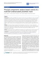
Figure 1 Hidden Markov Model for ancestry inference. Each individual’s local ancestral state probability, γ , is modeled as a function of
preceding ancestral state probabilities in each Markov chain, genetic distance to neighboring markers, d, individual global ancestry parameters and
observed haplotype or genotypes, a, in a region.

phased data set such as that provided by the International
HapMap Project [36], which can be found in the accompanying companion package, ALDdata. These methods
can be extended to unphased data, but phased data are
currently required by ALDsuite.
Higher order ancestral LD information is approximated
in this method using principal components (PCs) of the
surrounding, linked markers, and a principal component analysis (PCA) is performed. Samples from modernday surrogate populations chosen to represent ancestral,
admixing populations are analyzed in the PCA, and PCs
accounting for 80% of the observed variation are chosen to model the likelihood of each ancestral population
within each window. The transformation of the genotype
data using the PC loadings from the lth surrogate ancestral
population is illustrated in Equation 1 where the principal
component matrix for a window is the matrix multiplication of the phased haplotype matrix, A (one row per

chromosome, one column per marker in the haplotype)
with the eigenvector matrix, v:
PCl (A) = Avl .

(1)

A logistic Principal Component Regression (PCR) is
then performed to infer the likelihood of each ancestral

state within each window as a function of these PCs, and
the regression coefficients are used as starting points for
local ancestral state probability calculation in the HMM.
In the case of two ancestral populations, this simplifies to
a logistic regression (see Equation 2); a multinomial logistic regression is used to model admixture between more
than two populations (see Appendix).
log

P g = 1 |A
P g = 0 |A

= β · PC1 (A) + ε,

P g = 0 |A =

1
1 + eβ·PC1 (A)

,

(2)

P g = 1 |A = 1 − P g = 0 |A ,
where g indicates the proposed ancestral population the
haplotype originated from. In sparsely sampled regions,
where only one marker was sampled within the bounds of
the window, observed alleles are used in the model instead
of PCR.
HMM algorithm

The HMM is an iterative, two-step process: in the first
step, ancestral state probabilities, γ , are calculated for
each individual in the sample at each window, followed in
the second step by an update of the parameters on which


Johnson et al. BMC Genetics (2015) 16:23

Page 4 of 11

γ is conditioned (see Figure 1). A basic overview is given
here; complete details are given in the Appendix section.
We calculate ancestral state probabilities using a
forward-backward algorithm similar to other admixture
HMMs [10-12], but using the PC loadings discussed
above to account for local LD. The ancestral state probabilities in each Markov chain (i.e. one starting at each
end of the chromosome, called the forward and reverse
chains) consist of the ancestral state probabilities defined
in Equation 2, conditioned on the ancestral state probability of the previous marker in the chain and the likelihood
of recombination between the two:
γ1 = P g1 |A

γj = P gj |A ∗ P rj G + 1 − P rj

γj−1 ,

(3)

where γj is a vector of ancestral state probabilities for the
jth window, P(g |A ) is defined in Equation 2, G is the global
ancestry or proportion of the genome inherited from
each ancestral population, and P(r) is the probability of
recombination between the midpoints of the current and
previous windows. These probabilities are further dependent on the number of generations since admixture, and
the genetic distance between window midpoints, d. The
product of the forward and reverse Markov chains, γf and
γr , is normalized (so that they sum to one) to obtain the
final ancestral state probabilities for each window, conditional on admixture linkage disequilibrium with nearby
windows,
γ = γf ∗ γr

.

(4)

The local ancestral state at each window is sampled using these ancestral state probabilities. Parameters
informing the HMM, particularly those on which γ is conditioned (e.g. PCR coefficients in Equation 2, estimated
global ancestry and estimated number of generations
since admixture), are updated at the conclusion of each
iteration, using the sampled ancestral states discussed in
the preceding paragraphs (see Appendix section for more
details).

ALDsuite retains computation efficiency as the number and density of markers increases by analyzing PCs
of small chromosomal regions. Additional computational
efficiency can be achieved in multicore environments with
support for the parallelization of ALDsuite using a distributed MCMC approach in which a separate analysis, or
chain, is run for each parallel process [37,38]. In order to
avoid unnecessary duplication of effort during the burn-in
phase, each chain reports back to the main process after
each iteration, where a remote proposal of each parameter is calculated based on the average of all parallel chains.

Each chain then updates its own local parameter space
using a weighted sum of the local and remote proposals:
iter
∗ local proposal +
n burn

1−

iter
n burn

∗ remote proposal,

(5)
where iter is the current iteration and n burn is the total
number of burn-in iterations. This results in a quicker
convergence to the equilibrium distribution while allowing each chain to start sampling at an independent state.
Error checking
Marker checks

Several quality control checks can be performed on each

marker using ALDsuite to identify potential genotyping
errors, mapping errors, flipped markers and irregular variations in allele frequency:
1. Hardy-Weinberg Equilibrium is tested using the
hwexact() function in the hwde package [39].
2. Markers with a missing data rate exceeding a
user-defined threshold are screened (default
threshold is 5%).
3. Allele frequencies from genotypic data coded as
A/C/T/G are compared among populations to
identify potential A-T/G-C flips that may have
occurred in data originating from different sources.
The default is to drop these markers from the
analysis set.
4. Allele frequencies in the admixed population are
compared with modern-day, ancestral surrogate
population allele frequencies to identify potentially
irregular loci.
Individual checks

ALDsuite also includes several quality control checks for
individuals, to identify potentially bad samples which the
user may wish to remove:
1. Individuals with a missing data rate exceeding a
user-defined threshold are screened (default
threshold is 5%).
2. When sex chromosome data are available, simple
gender checks are performed and possible issues are
flagged.
3. The sample is screened for potentially related
individuals, and matches are flagged.

Parameter checks

The parameter state space can be saved at each iteration
during the analysis for evaluation of convergence.
1. A function is provided to graphically display the
desired parameters over the course of the burnin and
follow-on phases of the analysis. Greater parameter


Johnson et al. BMC Genetics (2015) 16:23

Page 5 of 11

variability can be expected during the burnin phase,
and multiple MCMC chains can be compared to
evaluate how variable parameters are across
independent chains. Parameters who’s mean values
change significantly during the follow-on phase
indicate the need for a longer burnin phase.
2. To evaluate the representativeness of chosen
modern-day surrogate samples, the value of τ should
be checked (see Appendix section for more details).
Higher values indicate a better fit; instances where
τ < 50 − 100 either indicate poorly chosen
modern-day surrogates or the presence of allele flips.
In the analysis of African American data, using the
YRI and CEU HapMap data as modern-day surrogate
samples, we have observed τ ∈ (200 − 1000),
depending on the density of the marker set.
Statistical association

Local and global ancestry estimates across the genome
are reported for each individual. With this information
the user can use one of several statistical association
techniques for mapping disease genes and/or fine mapping of disease-associated loci. When mapping disease
genes by ALD, an association with local ancestry at a
locus is the primary association being tested. The caseonly regression model, defined in Equation 6, compares
the difference between local ancestry and global ancestry. Other data (e.g. case-control) can be similarly modeled as defined in Equation 7. In both of these models,
regions with statistically significant regression coefficients
for local ancestry are inferred to harbor disease modifying
genes.
global ancestry ∼ β0 + β1 (local ancestry) + β2 (covariates)
(6)

link(Y ) ∼ β0 + β1 (local ancestry) + β2 (global ancestry)
+ β3 (covariates)
(7)
When a disease locus is identified, a fine mapping analysis is needed to identify specific variants most strongly
associated with the disease outcome. In a fine mapping
analysis both ancestral and genotype data are included in
the model (see Equation 8), and an association between
genotype and disease is the primary association being
tested.
link(Y ) ∼ β0 + β1 (genotypes) + β2 (local ancestry)
+ β3 (global ancestry) + β4 (covariates)
(8)

These generalized linear models are very flexible, allowing for multiple types of disease phenotypes (e.g. continuous, dichotomous, time-to-event) and any covariates
deemed appropriate by the investigator. Wrapper functions for these models along with support for parallel
computation is included in ALDsuite.

Simulations and power
Control populations

Chromosomes with known ancestry at each marker were
simulated in a two step process: 1) recombination points
were assigned to each chromosome based on the number of generations since admixture; 2) chromosomal segments were randomly selected from the YRI and CEU
HapMap samples to fill in each chromosomal region, with
the probablility of sampling a given HapMap chromosome conditional upon the assigned global ancestry for
the simulted chromosome. In this way, admixed chromosomes were simulated with appropriate admixture linkage
patterns across the chromosome without regard to how
windows are chosen.
Random recombination rates, conditional upon the
number of generations since admixture, and global ancestral proportions, G, were sampled, and 400 chromosomes
were simulated. Values for the number of generations
since admixture were Gamma distributed with a mean of
6 and standard deviation of 2, and values for G were Beta
distributed with a mean of 0.82 and standard deviation of
0.1. These parameters were chosen to simulate a typical
African American sample. The CEU and YRI populations
were also used as modern-day representative populations,
but with the initial PCR estimates randomly modified to
simulate imperfect surrogates. This was done by adding
a normal random value to each of the regression estimates, the variance of which was scaled by each estimate’s
standard error.
A sample of 100 individuals from each simulation above
was analyzed using ALDsuite, MULTIMIX and PCAdmix [18,28], and the proportion of correct and incorrect
inferences are reported.
Empirical data

The ASW population from the International HapMap

Project, a sample of African Americans from the Southwest USA, were analyzed using YRI and CEU populations
as surrogate ancestral populations. These populations
were analyzed using ALDsuite as well as MULTIMIX
and PCAdmix [18,28], and a representative sample of the
results on chromosome 20 are shown.
Additional tools

Several tools are included in the R package, additional
to the local ancestry inference and disease association
statistics described above. These include input and output


Johnson et al. BMC Genetics (2015) 16:23

data formatting aids, quality control and analysis of the
data, and useful data sets. Formatting functions are available for generating prior parameter estimates for different
populations using HapMap populations contained in the
ALDdata package, and calculation of genetic distance in
humans is performed using one of several maps, including the International HapMap Project and those generated
by Matise et al. [36,40,41]. Error checking functions for
quality control measures discussed in the Error Checking section are included as well as some basic graphics.
Additional downstream statistical analysis and custom
generation of graphics using the diverse and powerful
toolset provided by R is also directly available [42].

Results and discussion
While sparse marker panels are more cost effective and
have proven powerful in the detection several important disease risk genes, dense data provide more accurate
ancestry inference and a finer resolution of recombination points [13]. One strategy that has been used is to
follow up a MALD study with fine typing around an associated locus [43]. With ALDsuite both sparse and dense

marker data are analyzed in combination, resulting in better global ancestry estimates, while being able to infer
local ancestry on a much finer scale in areas of particular
interest. This program should increase the utility of dense
marker datasets available from many large cohort studies
that include African Americans.
ALDsuite provides accurate inference of local ancestry, while indirectly modeling local, higher order LD
remaining from ancestral populations. The analysis of our
simulation resulted in 96.3% accuracy of local ancestry
inference, compared to the 98.1% accuracy of PCAdmix
and the 98.7% accuracy of MULTIMIX, which is on par
with other leading analysis software [16,32]. Comparison
of chromosomes from an analysis of the ASW population
using ALDsuite, MULTIMIX and PCAdmix also shows a

Page 6 of 11

good degree of concordance between the methods used
(see Figure 2).
One striking difference between the results shown in
Figure 2 are the differing window sizes. The binning of
markers in MULTIMIX and PCAdmix is done by arbitrarily grouping a fixed number of markers into each bin.
In more densely sampled areas, such as those closer to
the center of the chromosome, the window sizes are quite
small, while other less densely sampled areas have much
larger window sizes. The region at the beginning of the
chromosomes in Figure 2, for example, cover as much as
4 cM. Binning of markers in ALDsuite is done by genetic
distance, rather than the number of markers, creating a
more constant window size across the genome. In more
densely sampled regions, this helps maintain better computational properties, since fewer windows can be used to

cover the same region, while in sparsely sampled regions
a more precise estimate of the boundaries of ancestral
haplotypes can be obtained.
Another key feature of ALDsuite that all other densemarker admixture software lacks is direct access to statistical methods needed to map disease phenotypes. Not
only does ALDsuite provide utilities directly supporting
admixture mapping and fine mapping studies (see Implementation section), but many other proposed methods
can be easily implemented in R, using the output provided by ALDsuite [44-46]. Also, of eleven MALD studies
published in 2013 and early 2014, six used sparse marker
panels for disease gene mapping, at least two of which
explicitly thinned their dense marker data to accommodate the software used [47,48]. An additional 15 GWAS
studies we identified from 2013 used various software
listed in Table 1 to control for population substructure
resulting from admixture, mostly using dense marker
strategies (citations not listed here). This trend highlights
the need for a dense marker software package that, like
most sparse marker software, includes disease association
statistics for MALD.

Figure 2 Representative chromosomes from one individual in the ASW population. Local ancestry inference along chromosome 20 is shown
for ALDsuite (top), PCAdmix (middle) and MULTIMIX (bottom). A stacked bar plot indicating the inferred probability of African ancestry (represented
by green bars) and European ancestry (represented by blue bars) is given for each phased haplotype. The width of each bar is proportional to the
window size (in cM) covered by the markers used to infer ancestry.


Johnson et al. BMC Genetics (2015) 16:23

Conclusion
Admixture inference software can be categorized using a
few different metrics including the number of admixing
populations it can simultaneously infer, the way it models

local LD when analyzing dense marker data, the number
of admixing populations it will simultaneously infer and
support of disease gene mapping (see Table 1). There are
currently no software solutions which both offer analysis of dense marker data from more than two admixing
populations and disease association statistics, requiring
the use of several software programs, often with very different input and output data formats. ALDsuite offers a
fast, accurate estimation of global and local ancestry with
the tools needed from data quality control through mapping of disease genes, along with the rich statistical and
graphical utilities provided with R.

Availability and requirements
Project name: ALDsuite
Project homepage: />Operating systems(s): Windows, Mac, Linux
Programming language: R and C
Other Requirements: R, version 3.0 or greater with the
parallel, mvtnorm and hwde packages installed. The gdata
and ncdf R packages are also recommended.
License: GPL

Appendix
ALDsuite: Dense marker MALD using principal
components of ancestral linkage disequilibrium
Computational details for the algorithm used to sample
the joint distribution of the HMM for inferring local
ancestry. Throughout, parameters are indexed by i (individual), j (marker), c (chromosome) and k (ancestral
population).

Initialization of the parameter space
Distances, d, are calculated as the number of centimorgans to the previous marker, with each chromosome
starting with a missing value.

The modern allele frequencies on chromosome segments originating from ancestral populations, , parameterize the prior distribution of ancestral allele frequencies,
P. Eigen vectors for groups of markers used in modeling of ancestral LD within each ancestral population
are either given by the user or estimated from HapMap
data by the software. Prior estimates of logistic regression
coefficients, H, and their associated variance-covariance
matrices, , for inference of modern allele frequencies
as a function of nearby, linked markers are also either
provided by the user or estimated from HapMap data.
All associated markers within a user definable window
(default is 2 cM) are chosen to model ancestral LD, and

Page 7 of 11

the number of principal components, m-1, accounting for
80% of the genetic variation in each subset are chosen to
be included in the model, making a total of m coefficients,
including the intercept.
Initial values for ancestry, A, are obtained using a quick
frequentist algorithm, and global ancestry estimates for
each parent are initially equal.
Initial values for average number of generations since
admixture, λ, and effective population size of each prior
population, τ , can also be specified by the user. When
unspecified, default values tuned to the analysis of African
Americans are used.

MCMC Algorithm
Step 1. Sample Ancestral States

Ancestral state probabilities are calculated using a

forward-backward algorithm similar to that used by
admixture software for sparse marker sets [10-12]. The
main differences in our algorithm being that ancestral LD
is indirectly modeled, allowing analysis of dense marker
sets, and we estimate marginal ancestral state probabilities
for each inherited chromosome, requiring the genotype
data to be phased prior to analysis. These differences
motivate the majority of differences between our package
and other admixture software. In the forward portion of
the algorithm, ancestral state probabilities, γ , are calculated at each locus, dependent on the genotype at each
locus (probability that the ith individuals jth locus of chromosome c originated from the kth ancestral population).

γ =

P(a=x|g=k )P(g=k )
P(a=x)

P g=k

, a known
, a unknown

(A1)

Before we treat the probabilities in Equation A1, we note
that the probability of an observed recombination event,
rijc , over a distance of dj cM is a function of the number of
generations since admixture, λic :
P (r|λ = 1) =

1 − e−2d/100
,
2

P (r) = 1 −

1 + e−2d/100
2

(A2)
λ

(A3)

and the probability of any crossovers happening in one
haplotype since admixture over a window of size w cM
follows a Poisson distribution:
P (X > 0|w) = 1 − e−λw/100 .

(A4)

The probability of an individuals genotype at a locus,
a, conditional on the ancestral state, g, is a function of
the allele frequencies in each population and the principal


Johnson et al. BMC Genetics (2015) 16:23

Page 8 of 11

components of nearby, linked markers, spanning a region
of w cM.
1 − fj (a• , k, w) , x = 0
(A5)
P a = x|a• , g = k =
,x = 1
fj (a• , k, w)
fj (a• , k, d) = p ∗ P (X > 0|w) +
(A6)
logit−1 (β0 + β1 PC1 (a• ) + · · · )
(1 − P (X > 0|w)) ,
where the probability of one or more crossovers in the
haplotype block of w cM, which informs the principal
components regression, is defined in Equation A3, and
pjk is the allele frequency in chromosomes with k ancestry. We highlight the dependence of Equation A5 on the
probability of observing crossovers within the window
supporting the principal components regression. If there
is a crossover, the resulting haplotype is no longer representative of the ancestral population, and we rely upon the
allele frequency instead.
The probabilities of each ancestral state are further
dependent on the ancestral probabilities at the previous locus, γi(j−1)K , the distance, dj , between these loci
(missing if it is the first locus on a chromosome), the individuals recombination rates, λic , and the individuals global
ancestry, Aick (the distance between loci is in cM).
Now we treat the probability of the ancestral state, k, of
a locus, dependent on the ancestral state at the previous
locus in the Markov chain, k ∗ :
P g = k = A ∗ P (r) + γj−1 ∗ (1 − P (r)) .

(A7)

For the first locus on each chromosome, the only prior
information available is the global ancestry of the parents.
We essentially treat this scenario as if there were a known
recombination event, i.e. P(r1 ) = 1.
This also applies to the marginal probability of the
observed genotype, a, which depends Equation A4 and
Equation A7:
P a = x|g = k P g = k .

P (a = x) =

(A8)

k

The reverse chain is nearly identical, starting from the
opposite end of each chromosome and working back. The
final probabilities at each locus are obtained by multiplying the forward and reverse chains and normalizing,
γ = γf ∗ γr ,

(A9)

and a sample, G, of γ is taken for use in Step 2:
G ∼ Multinomial (γ ) .

(A10)

Step 2: Parameter Updates
Updates of A and AX , global ancestry

The prior of A is Dirichlet distributed and parameterized
by ω. The posterior is Dirichlet distributed, parameterized
by the sum of ω and γ , for all autosomal markers.

A ∼ Dirichlet (ω1 , . . . , ωK )
⎛
˙ ∼ Dirichlet ⎝ω1 +
A

⎞

(A11)

γK ⎠ (A12)

γ1 , . . . , ω K +
jc

jc

We accept the sampled values for each Metropolis˙ with probability
Hastings sample, A,
⎛
⎞
˙ ω−1
A
k
⎠.
min ⎝1,
(A13)

Aω−1
k

Patterson et. al. [11] have noted that sex chromosome
ancestry is highly correlated with autosomal chromosome ancestry. Sex chromosome ancestry proportions
are parameterized the same way here, by a scalar value,
omegaX , conditional on A. The posterior is Dirichlet distributed, parameterized by the product of A and ωX and
the sum of γ over the X chromosome.
AX ∼ Dirichlet ωX A
⎛

⎞

˙ X ∼ Dirichlet ⎝ωX A1 +
A

γK ⎠ (A15)

γ1 , . . . , ωX AK +
jc

(A14)

jc

We accept the sampled values for each Metropolis˙ X , with probability
Hastings sample, A
⎞
⎛
X

˙ X ω Ak −1
A
⎟
⎜
k
(A16)
min ⎝1,
X A −1 ⎠ .
ω
k
AX
k

Update of λ, mean number of generations since admixture

The prior of γ is Gamma distributed, parameterized by a
shape parameter, α1 and a rate parameter, α2 .
λ ∼ Gamma (α1 , α2 )

(A17)

The posterior is Gamma distributed:
⎛

⎞

λ˙ ∼ Gamma ⎝α1 + # crossovers, α2 +

d⎠ . (A18)
j

As noted in Equation A3, the number of crossovers is
Poisson distributed. To sample the number of crossovers
in each individual, conditional on there being at least 1
crossover, we generate a random uniform number for each
locus, qj , such that
qj ∈ P x = 0; λic , dj , 1

(A19)

and the number of corresponding crossovers for each
locus, nxj , such that
P x = nxj − 1; λic , dj < qj ≤ P x = nxj ; λic , dj .
(A20)


Johnson et al. BMC Genetics (2015) 16:23

Page 9 of 11

We then calculate the probability of 0 crossovers given
G, pxj0 , at each locus,
pxj0 = P x = 0 | Gic ; λic , dj
= 1 − P x > 0 | Gic ; λic , dj
where
P x > 0 | Gic ; λic , dj =

⎧
⎪
⎨

1
−λic dj

Aicg 1−e

⎪
⎩e−λic dj +Aicg

−λ d
1−e ic j

(A21)

.

(A22)
We keep the number of crossovers we sampled, nxj , at
that locus with probability 1 − pxj0 . The sum of these
sampled crossovers, we can sample the updated value, λ˙ ,
which we keep with probability
˙
λ˙ α1 −1 e−α2 λ
min 1, α −1 −α λ
λ 1 e 2

.

(A23)

Updates of p and β, parameterizing allele frequencies for
each population

The prior allele frequency of p is Beta distributed, parameterized by the product of τ and P. The posterior is Beta
distributed, parameterized by sum of the product of τ with
P and the number of reference/variant alleles sampled in
Step 2.
p ∼ Beta (τ P, τ (1 − P))

is a vector of the number of variant alleles and the
number of reference alleles in the modern-day ancestral
surrogate population sample. After each update of P, P˙ jk ,
the change is kept with probability
⎛

˙

min ⎝1,

k
k

˙

(τ P) (τ (1 − P))pτ P−1 (1 − p)τ (1−P)−1
(τ P) (τ (1 − P))pτ P−1 (1 − p)τ (1−P)−1

⎞
⎠.

(A31)
The prior of B is multivariate normally distributed as a
function of H and , as estimated from the modern-day
surrogate ancestral population.
B ∼ N H, diag ( ) I

(A32)

˙ are kept with probability
Sampled updates, B,
min 1, e

−τ 2
2

(β−B˙ )T (diag(

−1

)I)

(β−B˙ )−(β−B)T (diag(

−1

)I)

(β−B)

.

(A33)

τk 1 − Pjk + # variant alleles (A25)

The prior of τ is log normally distributed such that
log10 (τ ) has a mean of 2 and standard deviation of 0.5,

Each proportion is individually updated and is kept with
probability
⎛
⎞
p˙ τ P−1 (1 − p˙ )τ (1−P)−1
ic
⎠.
min ⎝1,
(A26)
pτ P−1 (1 − p)τ (1−P)−1
ic

For principal component regression modeling of the
allele probabilities, conditional on local ancestry, β is multivariate normally distributed, parameterized by the prior
B and the diagonal of . The posterior is additionally
parameterized by τ and the logistic regression coeffiˆ of the principal component regression model of
cients, β,
the haplotypes sampled at the end of Step 1.
1
β ∼ N B, 2 diag ( ) I
τ
nβˆ + τ B

1
β˙ ∼ N
,
diag ( ) I
n + τ (n + τ )2

(A27)

˙ )T (diag(
(β−B

−1

)I)

˙ )−(β−B)T (diag(
(β−B

log10 (τ ) ∼ N(2, 0.5).

(A34)

Samples values, τ˙ , are kept with respective probabilities,
min (1, LR (τ˙ , τ | p, P) ∗ LR (τ˙ , τ | β, B))

(A35)

where, given the length of β = l,
˙

LR (τ˙ , τ | p, P) =

k
k

˙

(τ P) (τ (1 − P))pτ P−1 (1 − p)τ (1−P)−1
(τ P) (τ (1 − P))pτ P−1 (1 − p)τ (1−P)−1

(A36)

LR (τ˙ , τ | β, B) =
jk

−l

τ˙
τ

e

τ 2 −τ˙ 2
2

−1

(β−B)T (diag( )I)

(β−B)

.

(A37)

(A28)
Update of ω and ωX , hyper parameters for A and AX

The prior of ω and ωX are log normally distributed, such
that log10 (ω) has mean 1 and standard deviation 0.5.

˙ is kept with probability
The sampled value, β,
−τ 2
2

(A30)

(A24)

p˙ jk ∼ Beta τk Pjk + # reference alleles,

min 1, e

The prior of P is Beta distributed, parameterized by the
number of observed alleles in the modern day equivalent
to the founder populations (e.g. Africans and Europeans
for African Americans).
P ∼ Beta ( )

, gijc = gi(j−1)c
, gijc = gi(j−1)c

Update of P, B and τ , hyper parameters for p and β

−1

)I)

(β−B)

.

(A29)

log10 (ω) ∼ N(1, 0.5)
X

log10 (ω ) ∼ N(1, 0.5)

(A38)
(A39)


Johnson et al. BMC Genetics (2015) 16:23

Page 10 of 11

Updated values for ω and ωX , ω˙ and ω˙ X , are kept with
probability

⎛

min ⎝1,

k
ic

⎛
⎜
min ⎝1,

k
ic

k

Aω˙ X
AωX

k
k
k

ω˙
ω

k
k

˙

(ω)Aω−1

(ω)A
˙ ω−1

(AωX ) AX
(Aω˙ X ) AX

Aω˙ X −1

⎞

4.

5.

⎠ , (A40)
⎞

6.

⎟
⎠ . (A41)
AωX −1
7.

Update of α, hyper parameters for λ

8.

Similar to other admixture software, updates of are a function of the mean of the Gamma distribution, α1 /α2 = m,
and the variance of the Gamma distribution, α1 /α22 = v.
Each is log normally distributed, such that log10 (m) and
log10 (v) each have mean 1 and standard deviation 0.5.
log10 (m) ∼ N(1, 0.5)

(A42)

log10 (v) ∼ N(1, 0.5)

(A43)

Values for m and v are updated independently, parameterized by α,
˙ and are kept with probability
⎞
⎛
(α1 )α˙ 2α˙ 1 λα˙ 1 −1 e−α˙ 2 λ
ic
⎠.
(A44)
min ⎝1,
(α˙ 1 )α2α1 λα1 −1 e−α2 λ
ic

Competing interests
The authors declare that they have no competing interests.

9.
10.

11.

12.

13.

14.

15.

Authors’ contributions
RCJ performed the majority of the programming and wrote the first manuscript
draft. GWN contributed to the admixture inference methods. RCJ, GWN, JFZ
and CAW contributed intellectually to the manuscript and development of the
software package. All authors read and approved the final manuscript.

16.

Acknowledgements
This project has been funded in whole or in part with federal funds from the
National Cancer Institute, National Institutes of Health, under contract
HHSN26120080001E. The content of this publication does not necessarily
reflect the views or policies of the Department of Health and Human Services,
nor does mention of trade names, commercial products, or organizations
imply endorsement by the U.S. Government. This Research was supported [in
part] by the Intramural Research Program of the NIH, National Cancer Institute,
Center for Cancer Research.

18.

Author details
1 BSP CCR Genetics Core, Leidos Biomedical Research, Inc, Frederick National
Laboratory, 21702 Frederick, MD, USA. 2 Chaire de Bioinformatique,
Conservatiore National des Arts et Metieèrs, 75003 Paris, France. 3 Basic
Research Laboratory, Leidos Biomedical Research, Inc, Frederick National
Laboratory, 21702 Frederick, MD, USA.
Received: 26 September 2014 Accepted: 6 February 2015

17.

19.

20.
21.

22.

23.

24.
25.

References
1. MacLean CJ, Workman PL. Genetic studies on hybrid populations. I.
Individual estimates of ancestry and their relation to quantitative traits.
Ann Human Genet. 1973;36(3):341–51.
2. Thoday JM. Limitations to genetic comparison of populations. J Biosocial
Sci. 1969;Suppl 1:3–14.
3. Seldin MF, Pasaniuc B, Price AL. New approaches to disease mapping in
admixed populations. Nature Reviews Genetics. 2011;12(8):523–8.

26.

27.
28.

Kopp JB, Smith MW, Nelson GW, Johnson RC, Freedman BI, Bowden
DW, et al. MYH9 is a Major-Effect Risk Gene for Focal Segmental
Glomerulosclerosis. Nat Genet. 2008;40(10):1175–84.
Nalls MA, Wilson JG, Patterson NJ, Tandon A, Zmuda JM, Huntsman S,
et al. Admixture mapping of white cell count: genetic locus responsible
for lower white blood cell count in the Health ABC and Jackson Heart
studies. Am J Human Genet. 2008;82(1):81–7.
Parker MM, Foreman MG, Abel HJ, Mathias RA, Hetmanski JB, Crapo JD,
et al., Admixture mapping identifies a quantitative trait locus associated
with FEV1/FVC in the COPDGene study. Genet Epidemiol. 2014;37(7):
652–9.
McKeigue PM. Mapping genes underlying ethnic differences in disease
risk by linkage disequilibrium in recently admixed populations. Am J
Human Genet. 1997;60(1):188.
Parra EJ, Marcini A, Akey J, Martinson J, Batzer MA, Cooper R, et al.
Estimating African American admixture proportions by use of
population-specific alleles. Am J Human Genet. 1998;63(6):1839–51.
Smith MW, O’Brien SJ. Mapping by admixture linkage disequilibrium:
advances, limitations and guidelines. Nat Genet. 2005;6:623–32.
Hoggart CJ, Shriver MD, Kittles RA, Clayton DG, McKeigue PM. Design
and analysis of admixture mapping studies. Am J Human Genet.
2004;74(5):965–78.
Patterson N, Hattangadi N, Lane B, Lohmueller KE, Hafler DA,
Oksenberg JR, Hauser SL, Smith MW, O’Brien SJ, Altshuler D, Daly MJ,

Reich D. Methods for high-density admixture mapping of disease genes.
Am J Human Genet. 2004;74(5):979–1000.
Falush D, Stephens M, Pritchard JK. Inference of population structure
using multilocus genotype data: linked loci and correlated allele
frequencies. Genetics. 2003;164(4):1567–87.
Tang H, Coram M, Wang P, Zhu X, Risch N. Reconstructing genetic
ancestry blocks in admixed individuals. Am J Human Genet. 2006;79(1):
1–12.
Price AL, Weale ME, Patterson N, Myers SR, Need AC, Shianna KV, et al.
Long-range LD can confound genome scans in admixed populations. Am
J Human Genet. 2008;83(1):132–5.
Sundquist A, Fratkin E, Do CB, Batzoglou S. Effect of genetic divergence in
identifying ancestral origin using HAPAA. Genome Res. 2008;18(4):676–82.
Price AL, Tandon A, Patterson N, Barnes KC, Rafaels N, Ruczinski I, et al.
Sensitive detection of chromosomal segments of distinct ancestry in
admixed populations. PLoS Genet. 2009;5(6):1000519.
Baran Y, Pasaniuc B, Sankararaman S, Torgerson DG, Gignoux C, Eng C,
et al. Fast and accurate inference of local ancestry in Latino populations.
Bioinformatics. 2012;28(10):1359–67.
Churchhouse C, Marchini J. Multiway admixture deconvolution using
phased or unphased ancestral panels. Genet Epidemiol. 2013;37(1):1–12.
Maples BK, Gravel S, Kenny EE, Bustamante CD. RFMix: A Discriminative
Modeling Approach for Rapid and Robust Local-Ancestry Inference. Am J
Human Genet. 2013;93(2):278–88.
Pritchard JK, Stephens M, Donnelly P. Inference of population structure
using multilocus genotype data. Genetics. 2000;155(2):945–59.
McKeigue PM, Carpenter JR, Parra EJ, Shriver MD. Estimation of
admixture and detection of linkage in admixed populations by a Bayesian
approach: application to African-American populations. Ann Human
Genet. 2000;64(Pt 2):171–86.

McKeigue PM, Colombo M, Agakov F, Datta I, Levin A, Favro D, et al.
Extending admixture mapping to nuclear pedigrees: application to
sarcoidosis. Genet Epidemiol. 2013;37(3):256–66.
Tang H, Peng J, Wang P, Risch NJ. Estimation of individual admixture:
analytical and study design considerations. Genet Epidemiol. 2005;28(4):
289–301.
Sankararaman S, Sridhar S, Kimmel G. Estimating local ancestry in
admixed populations. Am J Human Genet. 2008;82(2):290–303.
Sankararaman S, Kimmel G, Halperin E, Jordan MI. On the inference of
ancestries in admixed populations. Genome Res. 2008;18(4):668–75.
Pasaniuc B, Sankararaman S, Kimmel G, Halperin E. Inference of
locus-specific ancestry in closely related populations. Bioinformatics.
2009;25(12):213–21.
Alexander DH, Novembre J, Lange K. Fast model-based estimation of
ancestry in unrelated individuals. Genome Res. 2009;19(9):1655–64.
Brisbin A, Bryc K, Byrnes J, Zakharia F, Omberg L, Degenhardt J, et al.
PCAdmix: Principal components-based assignment of ancestry along


Johnson et al. BMC Genetics (2015) 16:23

29.

30.

31.

32.
33.
34.

35.
36.
37.

38.

39.
40.

41.

42.
43.

44.
45.

46.
47.

48.

each chromosome in individuals with admixed ancestry from two or
more populations. Human Biol. 2012;84(4):343–64.
Hu Y, Willer C, Zhan X, Kang HM, Abecasis GR. Accurate local-ancestry
inference in exome-sequenced admixed individuals via off-target
sequence reads. Am J Human Genet. 2013;93(5):891–99.
Loh P-R, Lipson M, Patterson N, Moorjani P, Pickrell JK, Reich D, et al.
Inferring admixture histories of human populations using linkage
disequilibrium. Genetics. 2013;193(4):1233–54.

Rodriguez JM, Bercovici S, Elmore M, Batzoglou S. Ancestry inference in
complex admixtures via variable-length Markov chain linkage models. J
Comput Biol. 2013;20(3):199–211.
Yang JJ, Li J, Buu A, Williams LK. Efficient inference of Local ancestry.
Bioinformatics. 2013;29(21):2750–6.
Zhang Y. De novo inference of stratification and local admixture in
sequencing studies. BMC Bioinf. 2013;14 Suppl 5:17.
Liu EY, Li M, Wang W, Li Y. MaCH-admix: genotype imputation for
admixed populations. Genet Epidemiol. 2013;37(1):25–37.
Guan Y. Detecting structure of haplotypes and local ancestry. Genetics.
2014;196(3):625–42.
International HapMap Consortium. A second generation human
haplotype map of over 3.1 million SNPs. Nature. 2007;449(7164):851–61.
Murray L. Distributed Markov chain Monte Carlo. In: LCCC: NIPS workshop
on learning on cores, clusters and clouds. Perth, Western Australia: CSIRO
Mathematics, Informatics and Statistics; 2010.
Wu X-L, Sun C, Beissinger TM, Rosa GJ, Weigel KA, Gatti NdL, et al.
Parallel Markov chain Monte Carlo - bridging the gap to
high-performance Bayesian computation in animal breeding and
genetics. Genet Sel Evol: GSE. 2012;44:29.
Maindonald JH. The hwde Package. 2013. />packages/hwde/.
Matise TC, Chen F, Chen W, De La Vega FM, Hansen M, He C, et al. A
second-generation combined linkage physical map of the human
genome. Genome Res. 2007;17(12):1783–6.
Nato AJ, Buyske S, Matise TC. The Rutgers Map: A third-generation
combined linkage-physical map of the human genome. 2014. http://
compgen.rutgers.edu/download_maps.shtml.
R Development Core Team. R: A language and environment for statistical
computing. Manual. 2013. .
Nelson GW, Freedman BI, Bowden DW, Langefeld CD, An P, Hicks PJ, et

al. Dense mapping of MYH9 localizes the strongest kidney disease
associations to the region of introns 13 to 15. Human Mol Genet.
2010;19(9):1805–15.
Zhu B, Ashley-Koch AE, Dunson DB. Generalized admixture mapping for
complex traits. G3 (Bethesda, Md.) 2013;3(7):1165–75.
Redden DT, Divers J, Vaughan LK, Tiwari HK, Beasley TM, Fernández JR,
et al. Regional admixture mapping and structured association testing:
conceptual unification and an extensible general linear model. PLoS
Genet. 2006;2(8):137.
Shriner D, Adeyemo A, Rotimi CN. Joint Ancestry and Association Testing
in Admixed Individuals. PLoS Comput Biol. 2011;7(12):1002325.
Kim-Howard X, Sun C, Molineros JE, Maiti AK, Chandru H, Adler A, et al.
Allelic heterogeneity in NCF2 associated with systemic lupus
erythematosus (SLE) susceptibility across four ethnic populations. Human
Mol Genet. 2013;23(6):1656–68.
Jeff JM, Armstrong LL, Ritchie MD, Denny JC, Kho AN, Basford MA, et al.
Admixture mapping and subsequent fine-mapping suggests a
biologically relevant and novel association on chromosome 11 for type 2
diabetes in African Americans. PloS One. 2014;9(3):86931.

Page 11 of 11

Submit your next manuscript to BioMed Central
and take full advantage of:
• Convenient online submission
• Thorough peer review
• No space constraints or color figure charges
• Immediate publication on acceptance
• Inclusion in PubMed, CAS, Scopus and Google Scholar
• Research which is freely available for redistribution

Submit your manuscript at
www.biomedcentral.com/submit