dynamic conditional random fields- factorized probabilistic models

Dynamic Conditional Random Fields: Factorized Probabilistic Models for
Labeling and Segmenting Sequence Data
Charles Sutton
Khashayar Rohanimanesh
Andrew McCallum
Department of Computer Science, University of Massachusetts, Amherst, MA 01003
Abstract
In sequence modeling, we often wish to repre-
sent complex interaction between labels, such
as when performing multiple, cascaded label-
ing tasks on the same sequence, or when long-
range dependencies exist. We present dynamic
conditional random fields (DCRFs), a general-
ization of linear-chain conditional random fields
(CRFs) in which each time slice contains a set
of state variables and edges—a distributed state
representation as in dynamic Bayesian networks
(DBNs)—and parameters are tied across slices.
Since exact inference can be intractable in such
models, we perform approximate inference us-
ing several schedules for belief propagation, in-
cluding tree-based reparameterization (TRP). On
a natural-language chunking task, we show that
a DCRF performs better than a series of linear-
chain CRFs, achieving comparable performance
using only half the training data.
1. Introduction
The problem of labeling and segmenting sequences of
observations arises in many different areas, including
bioinformatics, music modeling, computational linguistics,
speech recognition, and information extraction. Dynamic

Bayesian networks (DBNs) (Dean & Kanazawa, 1989;
Murphy, 2002) are a popular method for probabilistic se-
quence modeling, because they exploit structure in the
problem to compactly represent distributions over multi-
ple state variables. Hidden Markov models (HMMs), an
important special case of DBNs, are a classical method for
speech recognition (Rabiner, 1989) and part-of-speech tag-
ging (Manning & Sch
¨
utze, 1999). More complex DBNs
have been used for applications as diverse as robot naviga-
Appearing in Proceedings of the 21
st
International Conference
on Machine Learning, Banff, Canada, 2004. Copyright 2004 by
the first author.
tion (Theocharous et al., 2001), audio-visual speech recog-
nition (Nefian et al., 2002), activity recognition (Bui et al.,
2002), and information extraction (Skounakis et al., 2003;
Peshkin & Pfeffer, 2003).
DBNs are typically trained to maximize the joint probabil-
ity p(y, x) of a set of observation sequences x and labels
y. However, when the task does not require being able
to generate x, such as in segmenting and labeling, mod-
eling the joint distribution is a waste of modeling effort.
Furthermore, generative models often must make problem-
atic independence assumptions among the observed nodes
in order to achieve tractability. In modeling natural lan-
guage, for example, we may wish to use features of a word
such as its identity, capitalization, prefixes and suffixes,

neighboring words, membership in domain-specific lexi-
cons, and category in semantic databases like WordNet—
features which have complex interdependencies. Genera-
tive models that represent these interdependencies are in
general intractable; but omitting such features or modeling
them as independent has been shown to hurt accuracy (Mc-
Callum et al., 2000).
A solution to this problem is to model instead the condi-
tional probability distribution p(y|x). The random vector
x can include arbitrary, non-independent, domain-specific
feature variables. Because the model is conditional, the
dependencies among the features in x do not need to be
explicitly represented. Conditionally-trained models have
been shown to perform better than generatively-trained
models on many tasks, including document classification
(Taskar et al., 2002), part-of-speech tagging (Ratnaparkhi,
1996), extraction of data from tables (Pinto et al., 2003),
segmentation of FAQ lists (McCallum et al., 2000), and
noun-phrase segmentation (Sha & Pereira, 2003).
Conditional random fields (CRFs) (Lafferty et al., 2001)
are undirected graphical models that are conditionally
trained. Previous work on CRFs has focused on the linear-
chain structure, depicted in Figure 1, in which a first-order
Markov assumption is made among labels. This model
structure is analogous to conditionally-trained HMMs, and
has efficient exact inference algorithms. Often, however,
we wish to represent more complex interaction between
labels—for example, when longer-range dependencies ex-
ist between labels, when the state can be naturally repre-
sented as a vector of variables, or when performing mul-

tiple cascaded labeling tasks on the same input sequence
(which is prevalent in natural language processing, such as
part-of-speech tagging followed by noun-phrase segmenta-
tion).
In this paper, we introduce DynamicCRFs(DCRFs), which
are a generalization of linear-chain CRFs that repeat struc-
ture and parameters over a sequence of state vectors—
allowing us to represent distributed hidden state and com-
plex interaction among labels, as in DBNs, and to use
rich, overlapping feature sets, as in conditional models.
For example, the factorial structure in Figure 1(b) includes
links between cotemporal labels, explicitly modeling lim-
ited probabilistic dependencies between two different label
sequences. Other types of DCRFs can model higher-order
Markov dependence between labels (Figure 2), or incorpo-
rate a fixed-size memory. For example, a DCRF for part-of-
speech tagging could include for each word a hidden state
that is true if any previous word has been tagged as a verb.
Any DCRF with multiple state variables can be collapsed
into a linear-chain CRF whose state space is the cross-
product of the outcomes of the original state variables.
However, such a linear-chain CRF needs exponentially
many parameters in the number of variables. Like DBNs,
DCRFs represent the joint distribution with fewer parame-
ters by exploiting conditional independence relations.
Within natural-language processing, DCRFs are especially
attractive because they are a probabilistic generalization of
cascaded, weighted finite-state transducers (Mohri et al.,
2002). In general, many sequence-processing problems are
traditionally solved by chaining errorful subtasks such as

FSTs. In such an approach, however, errors early in pro-
cessing nearly always cascade through the chain, causing
errors in the final output. This problem can be solved
by jointly representing the subtasks in a single graphical
model, both explicitly representing their dependence, and
preserving uncertainty between them. DCRFs can repre-
sent dependence between subtasks solved using finite-state
transducers, such as phonological and morphological anal-
ysis, POS tagging, shallow parsing, and information extrac-
tion.
We evaluate DCRFs on a natural-language processing task.
A factorial CRF that learns to jointly predict parts of speech
and segment noun phrases performs better than cascaded
models that perform the two tasks in sequence. Also, we
compare several schedules for belief propagation on this
task, showing that although exact inference is feasible, ap-
proximate inference has lower total training time with no
loss in performance.
The rest of the paper is structured as follows. In section 2,
we describe the general framework of CRFs. Then, in sec-
x
t
x
t+1
x
t-1
y
t
y
t+1

y
t-1
w
t-1
x
t-1
x
t+1
x
t
y
t
y
t+1
y
t-1
w
t
w
t+1
(a)
(b)
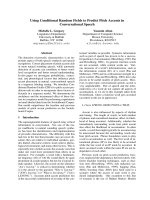
Figure 1. Graphical representation of (a) linear-chain CRF, and
(b) factorial CRF. Although the hidden nodes can depend on ob-
servations at any time step, for clarity we have shown links only
to observations at the same time step.
tion 3, we define DCRFs, and explain methods for approx-
imate inference and parameter estimation. In section 4, we
present the experimental results. We conclude in section 5.
2. CRFs

Conditional random fields (CRFs) (Lafferty et al., 2001)
are undirected graphical models that encode a conditional
probability distribution using a given set of features. CRFs
are defined as follows. Let G be an undirected model over
sets of random variables y and x. As a typical special case,
y = {y
t
} and x = {x
t
} for t = 1, . . . , T, so that y is a
labeling of an observed sequence x. If C = {{y
c
, x
c
}}
is the set of cliques in G, then CRFs define the conditional
probability of a state sequence given the observed sequence
as:
p
Λ
(y|x) =
1
Z(x)

c∈C
Φ(y
c
, x
c
), (1)

where Φ is a potential function and the partition function
Z(x) =

y

c∈C
Φ(y
c
, x
c
) is a normalization factor
over all state sequences for the sequence x. We assume
the potentials factorize according to a set of features {f
k
},
which are given and fixed, so that
Φ(y
c
, x
c
) = exp


k
λ
k
f
k
(y
c

, x
c
)

(2)
The model parameters are a set of real weights Λ = {λ
k
},
one weight for each feature.
Previous applications use the linear-chain CRF, in which
a first-order Markov assumption is made on the hidden
variables. A graphical model for this is shown in Fig-
ure 1. In this case, the cliques of the conditional model
are the nodes and edges, so that there are feature functions
f
k
(y
t−1
, y
t
, x, t) for each label transition. (Here we write
the feature functions as potentially depending on the entire
input sequence.) Feature functions can be arbitrary. For
example, a feature function f
k
(y
t−1
, y
t
, x, t) could be a bi-

nary test that has value 1 if and only if y
t−1
has the label
“adjective”, y
t
has the label “proper noun”, and x
t
begins
with a capital letter.
v
t-1
y
t-1
w
t-1
y
t-2
w
t-1
v
t-1
v
t
y
t
y
t-1
w
t
Factorial

y
t
y
t-1
Second-order Markov
v
t
y
t
w
t
Hierarchical
w
t-1
F
y
F
v
F
y
F
v
Figure 2. Examples of DCRFs. The dashed lines indicate the boundary between time steps.
3. Dynamic CRFs
3.1. Model Representation
A Dynamic CRF is a conditionally-trained undirected
graphical model whose structure and parameters are re-
peated over a sequence. As with a DBN, a DCRF can be
specified by a template that gives the graphical structure,
features, and weights for two time steps, which can then

be unrolled given an instance x. The same set of features
and weights is used at each sequence position, so that the
parameters are tied across the network. Several example
templates are given in Figure 2.
Now we give a formal description of the unrolling process.
Let y = {y
1
. . . y
T
} be a sequence of random vectors
y
i
= (y
i1
. . . y
im
). To give the likelihood equation for ar-
bitrary DCRFs, we require a way to describe a clique in the
unrolled graph independent of its position in the sequence.
For this purpose we introduce the concept of a clique in-
dex. Given a time t, we can denote any variable y
ij
in y by
two integers: its index j in the state vector y
i
, and its time
offset ∆t = i − t. We will call a set c = {(∆t, j)} of such
pairs a clique index, which denotes a set of variables y
t,c
by y

t,c
≡ {y
t+∆t,j
| (∆t, j) ∈ c}. That is, y
t,c
is the set of
variables in the unrolled version of clique index c at time t.
Now we can formally define DCRFs:
Definition Let C be a set of clique indices, F =
{f
k
(y
t,c
, x, t)} be a set of feature functions and Λ = {λ
k
}
be a set of real-valued weights. Then (C, F, Λ) is a DCRF
if and only if
p(y|x) =
1
Z(x)

t

c∈C
exp


k
λ

k
f
k
(y
t,c
, x, t)

(3)
where Z(x) =

y

t

c∈C
exp (

k
λ
k
f
k
(y
t,c
, x, t)) is
the partition function.
Although we define a DCRF has having the same set of
features for all the cliques, in practice, we choose feature
functions f
k

so that they are non-zero except on cliques
with some index c
k
. Thus, we will sometimes think of each
clique index has having its own set of features and weights,
and speak of f
k
and λ
k
as having an associated clique index
c
k
.
DCRFs generalize not only linear-chain CRFs, but more
complicated structures as well. For example, in this paper,
we use a factorial CRF (FCRF), which has linear chains
of labels, with connections between cotemporal labels. We
name these after factorial HMMs (Ghahramani & Jordan,
1997). Figure 1(b) shows an unrolled factorial CRF. Con-
sider an FCRF with L chains, where Y
,t
is the variable in
chain  at time t. The clique indices for this DCRF are of
the form {(0, ), (1, )} for each of the within-chain edges
and {(0, ), (0, +1)} for each of the between-chain edges.
The FCRF G defines a distribution over hidden states as:
p(y|x) =
1
Z(x)


T −1

t=1
L

=1
Φ

(y
,t
, y
,t+1
, x, t)


T

t=1
L−1

=1
Ψ

(y
,t
, y
+1,t
, x, t)

, (4)

where {Φ

} are the potentials over the within-chain edges,
{Ψ

} are the potentials over the between-chain edges, and
Z(x) is the partition function. The potentials factorize ac-
cording to the features {f
k
} and weights {λ
k
} of G as:
Φ

(y
,t
, y
,t+1
, x, t) = exp


k
λ
k
f
k
(y
,t
, y
,t+1

, x, t)

Ψ

(y
,t
, y
+1,t
, x, t) = exp


k
λ
k
f
k
(y
,t
, y
+1,t
, x, t)

More complicated structures are also possible, such as
semi-Markov CRFs, in which the state transition probabil-
ities depend on how long the chain has been in its current
state, and hierarchical CRFs, which are moralized versions
of the hierarchical HMMs of Fine et al. (1998).
1
As in
DBNs, this factorized structure can use many fewer param-

eters than the cross-product state space: even the two-level
FCRF we discuss below uses less than an eighth of the pa-
rameters of the corresponding cross-product CRF.
1
Hierarchical HMMs were shown to be DBNs by Murphy and
Paskin (2001).
3.2. Inference in DCRFs
Inference in a DCRF can be done using any inference
algorithm for undirected models. For an unlabeled se-
quence x, we typically wish to solve two inference prob-
lems: (a) computing the marginals p(y
t,c
|x) over all
cliques y
t,c
, and (b) computing the Viterbi decoding y
∗
=
arg max
y
p(y|x). The Viterbi decoding is used to label a
new sequence, and marginal computation is used for pa-
rameter estimation (Section 3.3).
Because marginal computation is needed during training,
inference must be efficient so that we can use large train-
ing sets even if there are many labels. The largest experi-
ment reported here required computing pairwise marginals
in 866,792 different graphical models: one for each train-
ing example in each iteration of a convex optimization al-
gorithm. Since exact inference can be expensive in com-

plex DCRFs, we use approximate methods. Here we de-
scribe approximate inference using loopy belief propaga-
tion.
Although belief propagation is exact only in certain spe-
cial cases, in practice it has been a successful approximate
method for general graphical models (Murphy et al., 1999;
Aji et al., 1998). In general, belief propagation algorithms
iteratively update a vector m = (m
u
(x
v
)) of messages be-
tween pairs of vertices x
u
and x
v
. The update from x
u
to
x
v
is given by:
m
u
(x
v
) ←

x
u

Φ(x
u
, x
v
)

x
t
=x
v
m
t
(x
u
), (5)
where Φ(x
u
, x
v
) is the potential on the edge (x
u
, x
v
). Per-
forming this update for one edge (x
u
, x
v
) in one direction
is called sending a message from x

u
to x
v
. Given a mes-
sage vector m, approximate marginals are computed as
p(x
u
, x
v
) ← κΦ(x
u
, x
v
)

x
t
=x
v
m
t
(x
u
)

x
w
=x
u
m

w
(x
v
),
(6)
where κ is a normalization factor.
At each iteration of belief propagation, messages can be
sent in any order, and choosing a good schedule can af-
fect how quickly the algorithm converges. We describe two
schedules for belief propagation: tree-based and random.
The tree-based schedule, also known as tree reparameteri-
zation (TRP) (Wainwright et al., 2001; Wainwright, 2002),
propagates messages along a set of cross-cutting spanning
trees of the original graph. At each iteration of TRP, a span-
ning tree T
(i)
∈ Υ is selected, and messages are sent in
both directions along every edge in T
(i)
, which amounts to
exact inference on T
(i)
. In general, trees may be selected
from any set Υ = {T } as long as the trees in Υ cover the
edge set of the original graph. In practice, we select trees
randomly, but we select first edges that have never been
used in any previous iteration.
The random schedule simply sends messages across all
edges in random order. To improve convergence, we arbi-
trarily order each edge e

i
= (s
i
, t
i
) and send all messages
m
s
i
(t
i
) before any messages m
t
i
(s
i
). Note that for a graph
with V nodes and E edges, TRP sends O(V ) messages per
BP iteration, while the random schedule sends O(E) mes-
sages.
To perform Viterbi decoding, we use the same propaga-
tion algorithms, except that the summation in Equation 5
is replaced by maximization. Also, the algorithms that
we have described apply to DCRFs with at most pairwise
cliques. Inference in DCRFs with larger cliques can be per-
formed straightforwardly using generalized versions of the
variational approaches in this section (Yedidia et al., 2000;
Wainwright, 2002).
3.3. Parameter Estimation in DCRFs
The parameter estimation problem is to find a set of

parameters Λ = {λ
k
} given training data D =
{x
(i)
, y
(i)
}
N
i=1
. More specifically, we optimize the con-
ditional log-likelihood
L(Λ) =

i
log p
Λ
(y
(i)
| x
(i)
). (7)
The derivative of this with respect to a parameter λ
k
asso-
ciated with clique index c is
∂L
∂λ
k
=


i

t
f
k
(y
(i)
t,c
, x
(i)
, t)
−

i

t

y
t,c
p
Λ
(y
t,c
| x
(i)
)f
k
(y
t,c

, x
(i)
, t).
(8)
where y
(i)
t,c
is the assignment to y
t,c
in y
(i)
, and y
t,c
ranges
over assignments to the clique y
t,c
. Observe that it is the
factor p
Λ
(y
t,c
| x
(i)
) that requires us to compute marginal
probabilities in the unrolled DCRF.
To reduce overfitting, we define a prior p(Λ) over parame-
ters, and optimize log p(Λ|D) = L(Λ) + log p(Λ). We use
a spherical Gaussian prior with mean µ = 0 and covariance
matrix Σ = σ
2

I, so that the gradient becomes
∂p(Λ|D)
∂λ
k
=
∂L
∂λ
k
−
λ
k
σ
2
.
See Peng and McCallum (2004) for a comparison of differ-
ent priors for linear-chain CRFs.
The function p(Λ|D) is convex, and can be optimized by
any number of techniques, as in other maximum-entropy
models (Lafferty et al., 2001; Berger et al., 1996). In the
results below, we use L-BFGS, which has previously out-
performed other optimization algorithms for linear-chain
CRFs (Sha & Pereira, 2003; Malouf, 2002).
The analysis above was for the fully-observed case, where
the training data include observed values for all variables in
2000 4000 6000 8000
87 88 89 90 91 92 93 94
Number of training instances
F1 on NP chunks
FCRF
Brill+CRF

CRF+CRF
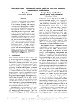
Figure 3. Performance of FCRFs and cascaded approaches on
noun-phrase chunking, averaged over five repetitions. The error
bars on FCRF and CRF+CRF indicate the range of the repetitions.
the model. If some nodes are unobserved, the optimization
problem becomes more difficult, because the log likelihood
is no longer convex in general (details omitted for space).
4. Experiments
We present experiments comparing factorial CRFs to other
approaches on noun-phrase chunking (Sang & Buchholz,
2000). Also, we compare different schedules of loopy be-
lief propagation in factorial CRFs.
4.1. Noun-Phrase Chunking
Automatically finding the base noun phrases in a sentence
can be viewed as a sequence labeling task by labeling
each word as either BEGIN-PHRASE, INSIDE-PHRASE, or
OTHER (Ramshaw & Marcus, 1995). The task is typically
performed by an initial pass of part-of-speech tagging, but
then it can be difficult to recover from errors by the tagger.
In this section, we address this problem by performing part-
of-speech tagging and noun-phrase segmentation jointly in
a single factorial CRF.
Our data comes from the CoNLL 2000 shared task (Sang
& Buchholz, 2000), and consists of sentences from the
Wall Street Journal annotated by the Penn Treebank project
(Marcus et al., 1993). We consider each sentence to be a
training instance, with single words as tokens. The data are
divided into a standard training set of 8936 sentences and
a test set of 2012 sentences. There are 45 different POS
labels, and the three NP labels.

We compare a factorial CRF to two cascaded approaches,
which we call CRF+CRF and Brill+CRF. CRF+CRF uses
one linear-chain CRF to predict POS labels, and another
linear-chain CRF to predict NP labels, using as a feature
the Viterbi POS labeling from the first CRF. Brill+CRF
Size CRF+CRF Brill+CRF FCRF
223 86.23 93.12
447 90.44 95.43
POS accuracy 670 92.33 N/A 96.34
894 93.56 96.85
2234 96.18 97.87
8936 98.28 98.92
223 92.67 93.75 93.87
447 94.09 94.91 95.03
NP accuracy 670 94.72 95.46 95.46
894 95.17 95.75 95.86
2234 96.08 96.38 96.51
8936 96.98 97.09 97.36
223 81.92 89.19
447 86.58 91.85
Joint accuracy 670 88.68 N/A 92.86
894 90.06 93.60
2234 93.00 94.90
8936 95.56 96.48
223 83.84 86.02 86.03
447 86.87 88.56 88.59
NP F1 670 88.19 89.65 89.64
894 89.21 90.31 90.55
2234 91.07 91.90 92.02
8936 93.10 93.33 93.87

Table 1. Comparison of performance of cascaded models and
FCRFs on simultaneous noun-phrase chunking and POS tag-
ging. The row CRF+CRF lists results from cascaded CRFs, and
Brill+CRF lists results from a linear-chain CRF given POS tags
from the Brill tagger. The FCRF always outperforms CRF+CRF,
and given sufficient training data outperforms Brill+CRF. With
small amounts of training data, Brill+CRF and the FCRF perform
comparably, but the Brill tagger was trained on over 40,000 sen-
tences, including some in the CoNLL 2000 test set.
predicts NP labels using the POS labels provided from the
Brill tagger, which we expect to be more accurate than
those from our CRF, because the Brill tagger was trained
on over four times more data, including sentences from the
CoNLL 2000 test set.
The factorial CRF uses the graph structure in Figure 1(b),
with one chain modeling the part-of-speech process and the
other modeling the noun-phrase process. We use L-BFGS
to optimize the posterior p(Λ|D), and TRP to compute the
marginal probabilities required by ∂L/∂λ
k
. Based on past
experience with linear-chain CRFs, we use the prior vari-
ance σ
2
= 10 for all models.
We factorize our features as f
k
(y
t,c
, x, t) =

p
k
(y
t,c
)q
k
(x, t) where p
k
(y
t,c
) is a binary function
on the assignment, and q
k
(x, t) is a function solely of
the input string. Table 2 shows the features we use. All
three approaches use the same features, with the obvious
exception that the FCRF and the first stage of CRF+CRF
do not use the POS features T
t
= T .
Performance on noun-phrase chunking is summarized in
Table 1. As usual, we measure performance on chunking
by precision, the percentage of returned phrases that are
w
t−δ
= w
w
t
matches [A-Z][a-z]+
w

t
matches [A-Z]
w
t
matches [A-Z]+
w
t
matches [A-Z]+[a-z]+[A-Z]+[a-z]
w
t
matches .*[0-9].*
w
t
appears in list of first names,
last names, company names, days,
months, or geographic entities
w
t
is contained in a lexicon of words
with POS T (from Brill tagger)
T
t
= T
q
k
(x, t + δ) for all k and δ ∈ [−3, 3]
Table 2. Input features q
k
(x, t) for the CoNLL data. In the above
w

t
is the word at position t, T
t
is the POS tag at position t, w
ranges over all words in the training data, and T ranges over all
part-of-speech tags.
correct; recall, the percentage of correct phrases that were
returned; and their harmonic mean F
1
. In addition, we also
report accuracy on POS labels,
2
accuracy on the NP labels,
and joint accuracy on (POS, NP) pairs. Joint accuracy is
simply the number of sequence positions for which all la-
bels were correct. The NP label accuracy should not be
compared across systems, because different systems use
different labeling schemes to encode which words are in
the same chunk.
Each row in Table 1 is the average of five different random
subsets of the training data, except for row 8936, which is
run on the single official CoNLL training set. All condi-
tions used the same 2012 sentences in the official test set.
On the full training set, FCRFs perform better on NP
chunking than either of the cascaded approaches, includ-
ing Brill+POS. The Brill tagger (Brill, 1994) is an estab-
lished high-performance tagger whose training set is not
only over four times bigger than the CoNLL 2000 data set,
but also includes the WSJ corpus from which the CoNLL
2000 test set was derived. The Brill tagger is 97% accu-

rate on the CoNLL data. Also, note that the FCRF—which
predicts both noun-phrase boundaries and POS—is more
accurate than a linear-chain CRF which predicts only part-
of-speech. We conjecture that the NP chain captures long-
run dependencies between the POS labels.
On smaller training subsets, the FCRF outperforms
CRF+CRF and performs comparably to Brill+CRF. For all
the training subset sizes, the difference between CRF+CRF
and the FCRF is statistically significant by a two-sample
t-test (p < 0.002). In fact, there was no subset of the
2
To simulate the effects of a cascaded architecture, the POS
labels in the CoNLL-2000 training and test sets were automati-
cally generated by the Brill tagger. Thus, POS accuracy measures
agreement with the Brill tagger, not agreement with human judge-
ments.
Method Time (hr) NP F1 LBFGS iter
µ s µ s µ
Random (3) 15.67 2.90 88.57 0.54 63.6
Tree (3) 13.85 11.6 88.02 0.55 32.6
Tree (∞) 13.57 3.03 88.67 0.57 65.8
Random (∞) 13.25 1.51 88.60 0.53 76.0
Exact 20.49 1.97 88.63 0.53 73.6
Table 3. Comparison of F1 performance on the chunking task by
inference algorithm. The columns labeled µ give the mean over
five repetitions, and s the sample standard deviation. Approx-
imate inference methods have labeling accuracy very similar to
exact inference with lower total training time. The differences
in training time between Tree (∞) and Exact and between Ran-
dom (∞) and Exact are statistically significant by a paired t-test

(df = 4; p < 0.005).
data on which CRF+CRF performed better than the FCRF.
The variation over the randomly selected training subsets
is small—the standard deviation over the five repetitions
has mean 0.39—indicating that the observed improvement
is not due to chance. Performance and variance on noun-
phrase chunking is shown in Figure 3.
On this data set, several systems are statistically tied for
best performance. Kudo and Matsumoto (2001) report an
F1 of 94.39 using a combination of voting support vector
machines. Sha and Pereira (2003) give a linear-chain CRF
that achieves an F1 of 94.38, using a second-order Markov
assumption, and including bigram and trigram POS tags as
features. An FCRF imposes a first-order Markov assump-
tion over labels, and represents dependencies only between
cotemporal POS and NP label, not POS bigrams or tri-
grams. Thus, Sha and Pereira’s results suggest that more
richly-structured DCRFs could achieve better performance
than an FCRF.
Other DCRF structures can be applied to many different
language tasks, including information extraction. Peshkin
and Pfeffer (2003) apply a generative DBN to extrac-
tion from seminar announcements (Frietag & McCallum,
1999), attaining improved results, especially in extracting
locations and speakers, by adding a factor to remember the
identity of the last non-background label. Our early results
with a similar structure seem promising, for example, one
DCRF structure performs within 2% F1 of a linear chain
CRF, despite being trained on 37% less data.
4.2. Comparison of Inference Algorithms

Because DCRFs can have rich graphical structure, and re-
quire many marginal computations during training, infer-
ence is critical to efficient training with many labels and
large data sets. In this section, we compare different infer-
ence methods both on training time and labeling accuracy
of the final model.
Because exact inference is feasible for a two-chain FCRF,
this provides a good case to test whether the final classifica-
tion accuracy suffers when approximate methods are used
to calculate the gradient. Also, we can compare different
methods for approximate inference with respect to speed
and accuracy.
We train factorial CRFs on the noun-phrase chunking task
described in the last section. We compute the gradient
using exact inference and approximate belief propagation
using random, and tree-based schedules, as described in
section 3.2. Algorithms are considered to have converged
when no message changes by more than 10
−3
. In these
experiments, the approximate BP algorithms always con-
verged, although this is not guaranteed in general. We
trained on five random subsets of 5% of the training data,
and the same five subsets were used in each condition. All
experiments were performed on a 2.8 GHz Intel Xeon with
4 GB of memory.
For each message-passing schedule, we compare terminat-
ing on convergence (Random(∞) and Tree(∞) in Table 3),
to terminating after three iterations (Random (3) and Tree
(3)). Although the early-terminating BP runs are less ac-

curate, they are faster, which we hypothesized could result
in lower overall training time. If the gradient is too inac-
curate, however, then the optimization will require many
more iterations, resulting in greater training time overall,
even though the time per gradient computation is lower.
Another hazard is that no maximizing step may be possi-
ble along the approximate gradient, even if one is possible
along the true gradient. In this case, the gradient descent al-
gorithm terminates prematurely, leading to decreased per-
formance.
Table 3 shows the average F1 score and total training times
of DCRFs trained by the different inference methods. Un-
expectedly, letting the belief propagation algorithms run
to convergence led to lower training time than the early
cutoff. For example, even though Random(3) averaged
427 sec per gradient computation compared to 571 sec
for Random(∞), Random(∞) took less total time to train,
because Random(∞) needed an average of 83.6 gradient
computations per training run, compared to 133.2 for Ran-
dom(3).
As for final classification performance, the various approx-
imate methods and exact inference perform similarly, ex-
cept that Tree(3) has lower final performance because max-
imization ended prematurely, averaging only 32.6 maxi-
mizer iterations. The variance in F1 over the subsets, al-
though not large, is much larger than the F1 difference be-
tween the inference algorithms.
Previous work (Wainwright, 2002) has shown that TRP
converges faster than synchronous belief propagation, that
is, with Jacobi updates. Both the schedules discussed in

section 3.2 use asynchronous Gauss-Seidel updates. We
emphasize that the graphical models in these experiments
are always pairs of coupled chains. On more complicated
models, or with a different choice of spanning trees, tree-
based updates could outperform random asynchronous up-
dates. Also, in complex models, the difference in classifi-
cation accuracy between exact and approximate inference
could be larger, but then exact inference is likely to be in-
tractable.
In summary, we draw three conclusions about this model.
First, using approximate inference instead of exact infer-
ence leads to lower overall training time with no loss in ac-
curacy. Second, there is little difference between a random
tree schedule and a completely random schedule for belief
propagation. Third, running belief propagation to conver-
gence leads both to increased classification accuracy and
lower overall training time than an early cutoff.
5. Conclusions
Dynamic CRFs are conditionally-trained undirected se-
quence models with repeated graphical structure and tied
parameters. They combine the best of both conditional
random fields and the widely successful dynamic Bayesian
networks (DBNs). DCRFs address difficulties of DBNs, by
easily incorporating arbitrary overlapping input features,
and of previous conditional models, by allowing more com-
plex dependence between labels. Inference in DCRFs can
be done using approximate methods, and training can be
done by maximum a posteriori estimation.
Empirically, we have shown that factorial CRFs can be
used to jointly perform several labeling tasks at once, shar-

ing information between them. Such a joint model per-
forms better than a model that does the individual label-
ing tasks sequentially, and has potentially many practical
implications, because cascaded models are ubiquitous in
NLP. Also, we have shown that using approximate infer-
ence leads to lower total training time with no loss in accu-
racy.
In future research, we plan to explore other inference meth-
ods to make training more efficient, including expectation
propagation (Minka, 2001) and variational approximations.
Also, investigating other DCRF structures, such as hier-
archical CRFs and DCRFs with memory of previous la-
bels, could lead to applications into many of the tasks to
which DBNs have been applied, including object recogni-
tion, speech processing, and bioinformatics.
Acknowledgments
We thank the three anonymous reviewers for many helpful com-
ments. This work was supported in part by the Center for In-
telligent Information Retrieval; by SPAWARSYSCEN-SD grant
number N66001-02-1-8903; by the Defense Advanced Research
Projects Agency (DARPA), through the Department of the Inte-
rior, NBC, Acquisition Services Division, under contract number
NBCHD030010; and by the Central Intelligence Agency, the Na-
tional Security Agency and National Science Foundation under
NSF grant # IIS-0326249. Any opinions, findings and conclu-
sions or recommendations expressed in this material are the au-
thors’ and do not necessarily reflect those of the sponsors.
References
Aji, S., Horn, G., & McEliece, R. (1998). The convergence of
iterative decoding on graphs with a single cycle. Proc. IEEE

Int’l Symposium on Information Theory.
Berger, A. L., Pietra, S. A. D., & Pietra, V. J. D. (1996). A max-
imum entropy approach to natural language processing. Com-
putational Linguistics, 22, 39–71.
Brill, E. (1994). Some advances in rule-based part of speech tag-
ging. Proceedings of the Twelfth National Conference on Arti-
ficial Intelligence (AAAI-94).
Bui, H. H., Venkatesh, S., & West, G. (2002). Policy recognition
in the Abstract Hidden Markov Model. Journal of Artificial
Intelligence Research, 17.
Dean, T., & Kanazawa, K. (1989). A model for reasoning about
persistence and causation. Computational Intelligence, 5(3),
142–150.
Fine, S., Singer, Y., & Tishby, N. (1998). The hierarchical hidden
Markov model: Analysis and applications. Machine Learning,
32, 41–62.
Frietag, D., & McCallum, A. (1999). Information extraction with
HMMs and shrinkage. AAAI Workshop on Machine Learning
for Information Extraction.
Ghahramani, Z., & Jordan, M. I. (1997). Factorial hidden Markov
models. Machine Learning, 245–273.
Kudo, T., & Matsumoto, Y. (2001). Chunking with support vector
machines. Proceedings of NAACL-2001.
Lafferty, J., McCallum, A., & Pereira, F. (2001). Conditional
random fields: Probabilistic models for segmenting and label-
ing sequence data. Proc. 18th International Conf. on Machine
Learning.
Malouf, R. (2002). A comparison of algorithms for maximum en-
tropy parameter estimation. Proceedings of the Sixth Confer-
ence on Natural Language Learning (CoNLL-2002) (pp. 49–

55).
Manning, C. D., & Sch
¨
utze, H. (1999). Foundations of statistical
natural language processing. Cambridge, MA: The MIT Press.
Marcus, M. P., Santorini, B., & Marcinkiewicz, M. A. (1993).
Building a large annotated corpus of English: The Penn Tree-
bank. Computational Linguistics, 19, 313–330.
McCallum, A., Freitag, D., & Pereira, F. (2000). Maximum en-
tropy Markov models for information extraction and segmenta-
tion. Proc. 17th International Conf. on Machine Learning (pp.
591–598). Morgan Kaufmann, San Francisco, CA.
Minka, T. (2001). A family of algorithms for approximate
Bayesian inference. Doctoral dissertation, MIT.
Mohri, M., Pereira, F., & Riley, M. (2002). Weighted finite-state
transducers in speech recognition. Computer Speech and Lan-
guage, 16, 69–88.
Murphy, K., & Paskin, M. A. (2001). Linear time inference in
hierarchical HMMs. Proceedings of Fifteenth Annual Confer-
ence on Neural Information Processing Systems.
Murphy, K. P. (2002). Dynamic Bayesian Networks: Representa-
tion, inference and learning. Doctoral dissertation, U.C. Berke-
ley.
Murphy, K. P., Weiss, Y., & Jordan, M. I. (1999). Loopy belief
propagation for approximate inference: An empirical study.
Fifteenth Conference on Uncertainty in Artificial Intelligence
(UAI) (pp. 467–475).
Nefian, A., Liang, L., Pi, X., Xiaoxiang, L., Mao, C., & Murphy,
K. (2002). A coupled HMM for audio-visual speech recogni-
tion. IEEE Int’l Conference on Acoustics, Speech and Signal

Processing (pp. 2013–2016).
Peng, F., & McCallum, A. (2004). Accurate information ex-
traction from research papers using conditional random fields.
Proceedings of Human Language Technology Conference and
North American Chapter of the Association for Computational
Linguistics (HLT-NAACL’04).
Peshkin, L., & Pfeffer, A. (2003). Bayesian information extrac-
tion network. Proceedings of the International Joint Confer-
ence on Artificial Intelligence (IJCAI).
Pinto, D., McCallum, A., Wei, X., & Croft, W. B. (2003). Table
extraction using conditional random fields. Proceedings of the
ACM SIGIR.
Rabiner, L. (1989). A tutorial on hidden Markov models and se-
lected applications in speech recognition. Proceedings of the
IEEE, 77, 257 – 286.
Ramshaw, L. A., & Marcus, M. P. (1995). Text chunking using
transformation-based learning. Proceedings of the Third ACL
Workshop on Very Large Corpora.
Ratnaparkhi, A. (1996). A maximum entropy model for part-of-
speech tagging. Proc. of the 1996 Conference on Empirical
Methods in Natural Language Proceeding (EMNLP 1996).
Sang, E. F. T. K., & Buchholz, S. (2000). Introduction to the
CoNLL-2000 shared task: Chunking. Proceedings of CoNLL-
2000 and LLL-2000. See .
be/˜erikt/research/np-chunking.html.
Sha, F., & Pereira, F. (2003). Shallow parsing with conditional
random fields. Proceedings of HLT-NAACL 2003.
Skounakis, M., Craven, M., & Ray, S. (2003). Hierarchical hidden
Markov models for information extraction. Proceedings of the
18th International Joint Conference on Artificial Intelligence.

Taskar, B., Abbeel, P., & Koller, D. (2002). Discriminative prob-
abilistic models for relational data. Eighteenth Conference on
Uncertainty in Artificial Intelligence (UAI02).
Theocharous, G., Rohanimanesh, K., & Mahadevan, S. (2001).
Learning hierarchical partially observable Markov decision
processes for robot navigation. Proceedings of the IEEE Con-
ference on Robotics and Automation.
Wainwright, M. (2002). Stochastic processes on graphs with cy-
cles: geometric and variational approaches. Doctoral disser-
tation, MIT.
Wainwright, M., Jaakkola, T., & Willsky, A. (2001). Tree-based
reparameterization for approximate estimation on graphs with
cycles. Advances in Neural Information Processing Systems
(NIPS).
Yedidia, J., Freeman, W., & Weiss, Y. (2000). Generalized be-
lief propagation. Advances in Neural Information Processing
Systems (NIPS).