kernel methods in machine learning
Bạn đang xem bản rút gọn của tài liệu. Xem và tải ngay bản đầy đủ của tài liệu tại đây (592.05 KB, 53 trang )
arXiv:math/0701907v3 [math.ST] 1 Jul 2008
The Annals of Statistics
2008, Vol. 36, No. 3, 1171–1220
DOI:
10.1214/009053607000000677
c
Institute of Mathematical Statistics, 2008
KERNEL METHODS IN MACHINE LEARNING
1
By Thomas Hofmann, Bernhard Sch
¨
olkopf
and Alexand er J. Smola
Darmstadt University of Technology, Max Planck Institute for Biological
Cybernetics and National ICT Australia
We review machine learning methods employing positive definite
kernels. These methods formulate learning and estimation problems
in a reproducing kernel Hilbert space (RKHS) of functions defined
on the data domain, expanded in terms of a kernel. Working in linear
spaces of function h as the benefit of facilitating the construction and
analysis of learning algorithms while at the same time allowing large
classes of functions. The latter include nonlinear functions as well as
functions defined on nonvectorial data.
We cover a wide range of methods, ranging from binary classifiers
to sophisticated methods for estimation with structured data.
1. Introduction. Over the last ten years estimation and learning meth-
ods utilizing positive definite kernels have become rather popular, particu-
larly in machine learning. Since these methods have a stronger mathematical
slant than earlier machine learning methods (e.g., neural networks), there
is also significant interest in the statistics and mathematics community for
these methods . The present review aims to summarize the state of the art on
a conceptual level. In doing so, we build on various sources, including Burges
[
25], Cristianini and Shawe-Taylor [37], Herbrich [64] and Vapnik [141] and,
in particular, Sch¨olkopf and Smola [
118], but we also add a fair amount of
more recent material which helps unifying the exposition. We have not had
space to include proofs; they can be foun d either in the lon g version of the
present paper (see Hofmann et al. [
69]), in the references given or in the
above books.
The main idea of all the described methods can be summarized in one
paragraph. Traditionally, theory and algorithms of machine learning and
Received December 2005; revised February 2007.
1
Supported in part by grants of the ARC and by the Pascal Network of Excellence.
AMS 2000 subject classifications. Primary 30C40; secondary 68T05.
Key words and phrases. Machine learning, reproducing kernels, support vector ma-
chines, graphical models.
This is an electronic reprint of the original article published by the
Institute of Mathematical Statistics in The Annals of Statistics,
2008, Vol. 36, No. 3, 1171–12 20. This reprint differs from the original in
pagination and typographic detail.
1
2 T. HOFMANN, B. SCH
¨
OLKOPF AND A. J. SMOLA
statistics has been very well developed for the linear case. Real world data
analysis problems, on the other hand, often require nonlinear methods to de-
tect the kind of dependencies that allow successful prediction of properties
of interest. By using a positive definite kernel, one can sometimes have the
best of both worlds. The kernel corresponds to a dot product in a (usually
high-dimensional) feature space. In this space, our estimation methods are
linear, but as long as we can formulate everything in term s of kernel evalu-
ations, we never explicitly have to compute in the high-dimensional feature
space.
The paper has three main sections: Section
2 deals with fundamental
properties of kernels, with special emphasis on (conditionally) positive defi-
nite kernels and their characterization. We give concrete examples for such
kern els and discus s kernels and reproducing kernel Hilbert spaces in the con-
text of regularization. Section
3 presents various approaches for estimating
dependencies and analyzing data that make use of kernels. We provide an
overview of the problem formulations as well as their solution using convex
programming techniques. Finally, Section
4 examines the us e of reproduc-
ing kernel Hilbert spaces as a means to define statistical models, the focus
being on structured , multidimensional responses. We also show how such
techniques can be combined with Markov networks as a suitable framework
to model depend en cies between response variables.
2. Kernels.
2.1. An introductory example. Suppose we are given empirical data
(x
1
, y
1
), . . . , (x
n
, y
n
) ∈ X × Y.(1)
Here, the domain X is some nonempty set that the inputs (the predictor
variables) x
i
are taken from; the y
i
∈ Y are called targets (the response var i-
able). Here and below, i, j ∈ [n], where we use the notation [n] := {1, . . . , n}.
Note that we h ave n ot made any assumptions on the domain X other
than it being a set. In order to study the problem of learning, we need
additional structure. In learning, we want to be able to generalize to unseen
data points. In the case of binary pattern recognition, given some n ew input
x ∈ X, we want to predict the corresponding y ∈ {±1} (more complex output
domains Y will be treated below). Loosely speaking, we want to choose y
such that (x, y) is in some sense similar to the training examples. To this
end, we need similarity measures in X and in {±1}. The latter is easier,
as two target values can only be identical or different. For the former, we
require a function
k : X × X → R, (x, x
′
) → k(x, x
′
)(2)
KERNEL METHODS IN MACHINE LEARNING 3
Fig. 1. A simple geometric classification algorithm: given two classes of points (de-
picted by “o” and “+”), com pute their means c
+
, c
−
and assign a test input x to the
one whose mean is closer. This can be done by looking at the dot product between x − c
[where c = ( c
+
+ c
−
)/2] and w := c
+
− c
−
, which changes sign as the enclosed angle passes
through π/2. Note that the corresponding decision boundary is a hyperplane (the dotted
line) orthogonal to w (from Sch¨olkopf and Smola [
118]).
satisfying, for all x, x
′
∈ X ,
k(x, x
′
) = Φ(x), Φ(x
′
),(3)
where Φ maps into some dot product space H, sometimes called the feature
space. The similarity measure k is usually called a kernel, and Φ is called its
feature map.
The advantage of using such a kernel as a similarity measure is that
it allows us to construct algorithms in dot product spaces. For instance,
consider the following simple classification algorithm, described in Figure
1,
where Y = {±1}. The idea is to compute the means of the two classes in
the feature space, c
+
=
1
n
+
{i:y
i
=+1}
Φ(x
i
), and c
−
=
1
n
−
{i:y
i
=−1}
Φ(x
i
),
where n
+
and n
−
are th e number of examples with positive and negative
target values, respectively. We then assign a new point Φ(x) to th e class
whose mean is closer to it. This leads to the prediction rule
y = sgn(Φ(x), c
+
− Φ(x),c
−
+ b)(4)
with b =
1
2
(c
−
2
− c
+
2
). Substituting the expressions for c
±
yields
y = sgn
1
n
+
{i:y
i
=+1}
Φ(x), Φ(x
i
)
k(x,x
i
)
−
1
n
−
{i:y
i
=−1}
Φ(x), Φ(x
i
)
k(x,x
i
)
+ b
,(5)
where b =
1
2
(
1
n
2
−
{(i,j):y
i
=y
j
=−1}
k(x
i
, x
j
) −
1
n
2
+
{(i,j):y
i
=y
j
=+1}
k(x
i
, x
j
)).
Let us consider one well-known special case of this type of classifier. As-
sume that the class means have the same distance to the origin (hence,
b = 0), and th at k(·, x) is a dens ity for all x ∈ X . If the two classes are
4 T. HOFMANN, B. SCH
¨
OLKOPF AND A. J. SMOLA
equally likely and were generated from two probability distributions that
are estimated
p
+
(x) :=
1
n
+
{i:y
i
=+1}
k(x, x
i
), p
−
(x) :=
1
n
−
{i:y
i
=−1}
k(x, x
i
),(6)
then (
5) is the es timated Bayes decision rule, plugging in the estimates p
+
and p
−
for the true densities.
The classifier (
5) is closely related to the Support Vector Machine (SVM )
that we w ill discuss below . It is linear in the feature space (
4), while in the
input domain, it is represented by a kernel expansion (
5). In both cases, the
decision boundary is a hyperplane in the feature space; however, the normal
vectors [for (
4), w = c
+
− c
−
] are usually rather different.
The normal vector not on ly characterizes the alignment of the hyperplane,
its length can also be used to construct tests for the equality of the two class-
generating distributions (Borgwardt et al. [
22]).
As an aside, note that if we normalize the targets such that ˆy
i
= y
i
/|{j :y
j
=
y
i
}|, in wh ich case the ˆy
i
sum to zero, then w
2
= K, ˆyˆy
⊤
F
, w here ·, ·
F
is the Froben ius dot p roduct. If the two classes have equal size, then up to a
scaling factor involving K
2
and n, this equals the kernel-target alignment
defined by Cristianini et al. [
38].
2.2. Positive definite kernels. We have required that a kernel s atisfy (3),
that is, correspond to a dot pro duct in some dot product space. In the
present section we show th at the class of kernels that can be written in the
form (
3) coincides with the class of positive definite kernels. This has far-
reaching consequences. There are examples of positive definite kernels which
can be evaluated efficiently even though they correspond to dot products in
infinite dimensional dot product spaces. In such cases, substituting k(x, x
′
)
for Φ(x), Φ(x
′
), as we have done in (
5), is crucial. In the machine learning
community, this substitution is called the kernel trick.
Definition 1 (Gram matrix). Given a kernel k and inputs x
1
, . . . , x
n
∈
X , the n × n matrix
K := (k(x
i
, x
j
))
ij
(7)
is called the Gram matrix (or kernel matrix) of k with respect to x
1
, . . . , x
n
.
Definition 2 (Positive definite matrix). A real n×n sy mmetric m atrix
K
ij
satisfying
i,j
c
i
c
j
K
ij
≥ 0(8)
for all c
i
∈ R is called positive definite. If equality in (
8) on ly occurs for
c
1
= ··· = c
n
= 0, then we shall call the matrix strictly positive definite.
KERNEL METHODS IN MACHINE LEARNING 5
Definition 3 (Positive definite kernel). Let X be a nonempty set. A
function k : X × X → R which for all n ∈ N, x
i
∈ X , i ∈ [n] gives rise to a
positive definite Gram matrix is called a positive definite kernel. A function
k : X × X → R which for all n ∈ N and distinct x
i
∈ X gives rise to a strictly
positive definite Gram matrix is called a strictly positive definite kernel.
Occasionally, we shall refer to positive definite kernels simply as kernels.
Note that, for simplicity, we have restricted ourselves to the case of real
valued kernels. However, with small changes, the below will also hold for the
complex valued case.
Since
i,j
c
i
c
j
Φ(x
i
), Φ(x
j
) =
i
c
i
Φ(x
i
),
j
c
j
Φ(x
j
) ≥ 0, kernels of the
form (
3) are positive definite for any choice of Φ. In particular, if X is already
a dot product space, we may choose Φ to be the identity. Kernels can thus be
regarded as generalized dot products. While they are not generally bilinear,
they sh are important properties with dot products, such as th e Cauchy–
Schwarz inequality: If k is a positive definite kernel, and x
1
, x
2
∈ X , th en
k(x
1
, x
2
)
2
≤ k(x
1
, x
1
) · k(x
2
, x
2
).(9)
2.2.1. Construction of the reproducing kernel Hilbert space. We now de-
fine a map from X into the space of functions mapping X into R, denoted
as R
X
, via
Φ : X → R
X
where x → k(·, x).(10)
Here, Φ(x) = k(·, x) denotes the function that assigns the value k(x
′
, x) to
x
′
∈ X .
We next construct a dot product space containing the images of the inputs
under Φ. To this end, we first turn it into a vector space by forming linear
combinations
f(·) =
n
i=1
α
i
k(·, x
i
).(11)
Here, n ∈ N, α
i
∈ R and x
i
∈ X are arbitrary.
Next, we define a dot product between f and another function g(·) =
n
′
j=1
β
j
k(·, x
′
j
) (w ith n
′
∈ N, β
j
∈ R and x
′
j
∈ X ) as
f, g :=
n
i=1
n
′
j=1
α
i
β
j
k(x
i
, x
′
j
).(12)
To see that this is well defined although it contains the expansion coefficients
and points, n ote that f, g =
n
′
j=1
β
j
f(x
′
j
). The latter, however, does not
depend on the particular expansion of f. Similarly, for g, note that f, g =
n
i=1
α
i
g(x
i
). This also shows that ·, · is bilinear. It is symmetric, as f, g =
6 T. HOFMANN, B. SCH
¨
OLKOPF AND A. J. SMOLA
g, f. Moreover, it is positive definite, since positive definiteness of k implies
that, for any function f , written as (
11), we have
f, f =
n
i,j=1
α
i
α
j
k(x
i
, x
j
) ≥ 0.(13)
Next, note that given functions f
1
, . . . , f
p
, and coefficients γ
1
, . . . , γ
p
∈ R, we
have
p
i,j=1
γ
i
γ
j
f
i
, f
j
=
p
i=1
γ
i
f
i
,
p
j=1
γ
j
f
j
≥ 0.(14)
Here, the equality follows from the bilinearity of ·, ·, and the right-hand
inequality from (
13).
By (
14), ·, · is a positive definite kernel, defined on our vector space of
functions. For the last step in proving that it even is a dot product, we note
that, by (
12), for all functions (11),
k(·, x), f = f(x) and, in particular, k(·, x), k(·, x
′
) = k(x, x
′
).(15)
By virtue of these properties, k is called a reproducing kernel (Aronszajn
[
7]).
Due to (
15) and (9), we have
|f(x)|
2
= |k(·, x), f|
2
≤ k(x, x) · f, f.(16)
By this inequality, f, f = 0 implies f = 0 , which is the last property that
was left to prove in order to establish that ·, · is a dot product.
Skipping some details, we add that one can complete the space of func-
tions (
11) in the norm corr esponding to the dot product, and thus gets a
Hilbert space H, called a reproducing kernel Hilbert space (RKHS).
One can define a RKHS as a Hilbert space H of functions on a set X with
the property that, for all x ∈ X and f ∈ H, the point evaluations f → f(x)
are continuous linear functionals [in particular, all point values f(x) are well
defined, which already distinguishes RKHSs from many L
2
Hilbert spaces].
From the point evaluation functional, one can then construct th e reproduc-
ing kernel using the Riesz repr esentation theorem. The Moore–Aronszajn
theorem (Aronszajn [
7]) states that, for every positive definite kernel on
X × X , there exists a unique RKHS and vice versa.
There is an analogue of the kernel trick for distances rather than dot
products, that is, dissimilarities rather than similarities. This leads to the
larger class of conditionally positive definite k ernels. Those kernels are de-
fined just like positive definite ones, with the one difference being that their
Gram matrices need to satisfy (8) only subject to
n
i=1
c
i
= 0.(17)
KERNEL METHODS IN MACHINE LEARNING 7
Interestingly, it turns out that many kernel algorithms, including SVMs and
kern el PCA (see Section
3), can be applied also with this larger class of
kern els, due to their being translation invariant in feature space (Hein et al.
[63] and Sch¨olkopf and Smola [118]).
We conclude this section with a note on terminology. In the early years of
kern el machine learning research, it was not the notion of p ositive definite
kern els that was being used. Instead, researchers considered kernels satis-
fying the conditions of Mercer’s theorem (Mercer [
99], see, e.g., Cristianini
and Shawe-Taylor [
37] and Vapnik [141]). However, while all such kernels do
satisfy (
3), the converse is not true. Since (3) is what we are interested in,
positive definite kernels are thus the right class of kernels to consider.
2.2.2. Properties of positive definite kernels. We begin with some closure
properties of the set of positive definite kernels.
Proposition 4. Below, k
1
, k
2
, . . . are arbitrary positive definite kernels
on X × X , where X is a nonempty set:
(i) The set of positive definite kernels is a closed convex cone, that is,
(a) if α
1
, α
2
≥ 0, then α
1
k
1
+ α
2
k
2
is positive definite; and (b) if k(x, x
′
) :=
lim
n→∞
k
n
(x, x
′
) exists for all x, x
′
, then k is positive definite.
(ii) The pointwise product k
1
k
2
is positive definite.
(iii) Assume that for i = 1, 2, k
i
is a positive definite kernel on X
i
× X
i
,
where X
i
is a nonempty set. Then the tensor product k
1
⊗ k
2
and the direc t
sum k
1
⊕ k
2
are positive definite kernels on (X
1
× X
2
) × (X
1
× X
2
).
The proofs can be f ou nd in Berg et al. [
18].
It is reassuring that sums and p roducts of positive definite kernels are
positive definite. We will now explain that, loosely speaking, there are no
other operations that preserve positive definiteness. To this end, let C de-
note the set of all functions ψ: R → R that map positive definite kernels to
(conditionally) positive definite kernels (readers who are not interested in
the case of conditionally positive definite kernels may ignore the term in
parentheses). We define
C := {ψ|k is a p.d. kernel ⇒ ψ(k) is a (conditionally) p.d. kernel},
C
′
= {ψ| for any Hilbert space F,
ψ(x, x
′
F
) is (conditionally) positive definite},
C
′′
= {ψ| for all n ∈ N: K is a p.d.
n × n matrix ⇒ ψ(K) is (conditionally) p.d.},
where ψ(K) is the n × n matrix with elements ψ(K
ij
).
8 T. HOFMANN, B. SCH
¨
OLKOPF AND A. J. SMOLA
Proposition 5. C = C
′
= C
′′
.
The following proposition follows from a result of FitzGerald et al. [
50] for
(conditionally) positive definite matrices; by Proposition
5, it also applies for
(conditionally) positive definite kernels, and for functions of dot products.
We state the latter case.
Proposition 6. Let ψ : R → R. Then ψ(x, x
′
F
) is positive definite for
any Hilbert space F if and only if ψ is real entire of the form
ψ(t) =
∞
n=0
a
n
t
n
(18)
with a
n
≥ 0 for n ≥ 0.
Moreover, ψ(x, x
′
F
) is conditionally positive definite for any Hilbert
space F if and only if ψ is real entire of the form (
18) with a
n
≥ 0 for
n ≥ 1.
There are further properties of k that can be read off the coefficients a
n
:
• Steinwart [
128] showed that if all a
n
are strictly positive, then th e ker-
nel of Proposition
6 is universal on every compact subset S of R
d
in the
sense that its RKHS is dense in the space of continuous functions on S in
the ·
∞
norm. For support vector machines using universal kernels, he
then shows (universal) consistency (Steinwart [129]). Examples of univer-
sal kernels are (
19) and (20) below.
• In Lemma
11 we will show that the a
0
term d oes not affect an SVM.
Hence, we infer that it is actually sufficient for consistency to have a
n
> 0
for n ≥ 1.
We conclude the section with an example of a kernel which is positive definite
by Proposition
6. To this end, let X be a d ot product space. The power series
expansion of ψ(x) = e
x
then tells us that
k(x, x
′
) = e
x,x
′
/σ
2
(19)
is positive definite (Haussler [
62]). If we further multiply k with the positive
definite kernel f (x)f(x
′
), where f (x) = e
−x
2
/2σ
2
and σ > 0, this leads to
the positive definiteness of the Gaussian kernel
k
′
(x, x
′
) = k(x, x
′
)f(x)f (x
′
) = e
−x−x
′
2
/(2σ
2
)
.(20)
KERNEL METHODS IN MACHINE LEARNING 9
2.2.3. Properties of positive definite fu nctions. We now let X = R
d
and
consider positive definite kernels of the form
k(x, x
′
) = h(x − x
′
),(21)
in which case h is called a positive definite fu nc tion. The following charac-
terization is due to Bochner [
21]. We state it in the f orm given by Wendland
[152].
Theorem 7. A continuous function h on R
d
is positive definite if and
only if there exists a finite nonnegative Bore l measure µ on R
d
such that
h(x) =
R
d
e
−ix,ω
dµ(ω).(22)
While normally formulated for complex valued functions, the theorem
also holds true for real functions. Note, however, that if we start with an
arbitrary nonnegative Borel measure, its Fourier transform may not be real.
Real-valued positive definite functions are distinguished by the fact that the
corresponding measur es µ are symmetric.
We may normalize h such that h(0) = 1 [hence, by (
9), |h(x)| ≤ 1 ], in
which case µ is a probability measure and h is its characteristic function. For
instance, if µ is a normal distribution of the form (2π/σ
2
)
−d/2
e
−σ
2
ω
2
/2
dω,
then the corresponding positive definite function is the Gaussian e
−x
2
/(2σ
2
)
;
see (20).
Bo chner’s theorem allows us to interpret the similarity measure k(x, x
′
) =
h(x − x
′
) in the frequency domain. The choice of the measure µ determines
which frequency components occur in the kernel. Since the solutions of kernel
algorithms will turn out to be finite kernel expansions, the measure µ will
thus determine which frequencies occur in the estimates, that is, it will
determine their regularization properties—more on that in Section
2.3.2
below .
Bo chner’s theorem generalizes earlier work of Mathias, and has itself been
generalized in various ways, that is, by Schoenberg [115]. An important
generalization considers Abelian semigroups (Berg et al. [18]). In that case,
the theorem p rovides an integral representation of positive definite functions
in terms of the semigroup’s semicharacters. Further generalizations were
given by Krein, for the cases of positive definite kernels and functions with
a limited number of negative squares. See Stewart [
130] for further details
and references.
As above, there are conditions that ensure that the positive definiteness
becomes strict.
Proposition 8 (Wendland [
152]). A positive definite function is strictly
positive de finite if the carrier of the measu re in its representation (22) con-
tains an open subset.
10 T. HOFMANN, B. SCH
¨
OLKOPF AND A. J. SMOLA
This implies that the Gaussian kernel is strictly positive definite.
An important special case of positive definite functions, which includes
the Gaussian, are radial basis functions. These are functions that can be
written as h(x) = g(x
2
) for some function g : [0, ∞[ → R. They have the
property of being invariant under the Euclidean group.
2.2.4. Examples of kernels. We have already seen several instances of
positive definite kernels, and now intend to complete our selection with a
few more examples. In particular, we discuss polynomial kernels, convolution
kern els, ANOVA expansions and kernels on documents.
Polynomial kernels. From Proposition
4 it is clear that homogeneous poly-
nomial kernels k(x, x
′
) = x, x
′
p
are positive definite for p ∈ N and x, x
′
∈ R
d
.
By direct calculation, we can derive the correspondin g feature m ap (Poggio
[
108]):
x, x
′
p
=
d
j=1
[x]
j
[x
′
]
j
p
(23)
=
j∈[d]
p
[x]
j
1
· ·· · · [x]
j
p
· [x
′
]
j
1
· ·· · · [x
′
]
j
p
= C
p
(x), C
p
(x
′
),
where C
p
maps x ∈ R
d
to the vector C
p
(x) whose entries are all possible
pth degree ord ered products of the entries of x (note that [d] is used as a
shorthand for {1, . . . , d}). The polynomial kernel of degree p thus compu tes
a dot p roduct in the space spanned by all monomials of degree p in th e input
co ordinates. Oth er useful kernels include the inhomogeneous polynomial,
k(x, x
′
) = (x, x
′
+ c)
p
where p ∈ N and c ≥ 0,(24)
which computes all monomials up to degree p.
Spline kernels. It is possible to obtain spline functions as a result of kernel
expansions (Vapnik et al. [
144] simply by noting that convolution of an even
number of indicator f unctions yields a p ositive kernel function. Denote by
I
X
the indicator (or characteristic) function on the set X, and denote by
⊗ the convolution operation, (f ⊗ g)(x) :=
R
d
f(x
′
)g(x
′
− x)dx
′
. Then the
B-spline kernels are given by
k(x, x
′
) = B
2p+1
(x − x
′
) where p ∈ N with B
i+1
:= B
i
⊗ B
0
.(25)
Here B
0
is the characteristic function on the unit ball in R
d
. From the
definition of (
25), it is obvious that, for odd m, we may write B
m
as the
inner product between functions B
m/2
. Moreover, note that, for even m, B
m
is not a kernel.
KERNEL METHODS IN MACHINE LEARNING 11
Convolutions and structures. Let us now move to kernels defined on struc-
tured objects (Haussler [
62] and Watkins [151]). Su ppose the object x ∈ X is
composed of x
p
∈ X
p
, where p ∈ [P ] (note that the s ets X
p
need n ot be equal).
For instance, consider the string x = AT G and P = 2. It is composed of the
parts x
1
= AT and x
2
= G, or alternatively, of x
1
= A and x
2
= T G. Math-
ematically speaking, th e set of “allowed” decompositions can be thought
of as a relation R(x
1
, . . . , x
P
, x), to be read as “x
1
, . . . , x
P
constitute the
composite obj ect x.”
Haussler [
62] investigated how to define a kernel between composite ob-
jects by building on similarity measures that assess their respective parts;
in other words, kernels k
p
defined on X
p
× X
p
. Define the R-convolution of
k
1
, . . . , k
P
as
[k
1
⋆ · · · ⋆ k
P
](x, x
′
) :=
¯x∈R(x),¯x
′
∈R(x
′
)
P
p=1
k
p
(¯x
p
, ¯x
′
p
),(26)
where the sum runs over all possible ways R(x) and R(x
′
) in which we
can decompose x into ¯x
1
, . . . , ¯x
P
and x
′
analogously [h ere we used the con-
vention that an empty sum equals zero, hence, if either x or x
′
cannot be
decomposed, then (k
1
⋆ ··· ⋆ k
P
)(x, x
′
) = 0]. If there is only a finite number
of ways, the relation R is called finite. In this case, it can be shown that the
R-convolution is a valid kernel (Haussler [
62]).
ANOVA kernels. Specific examples of convolution kernels are Gaussians
and ANOVA kernels (Vapnik [141] and Wahba [148]). To constru ct an ANOVA
kern el, we consider X = S
N
for some set S, and kernels k
(i)
on S × S, where
i = 1, . . . , N . For P = 1, . . . , N, the ANOVA kernel of order P is defined as
k
P
(x, x
′
) :=
1≤i
1
<···<i
P
≤N
P
p=1
k
(i
p
)
(x
i
p
, x
′
i
p
).(27)
Note th at if P = N , th e sum consists only of the term for which (i
1
, . . . , i
P
) =
(1, . . . , N), and k equals the tensor product k
(1)
⊗ · · · ⊗ k
(N)
. At the other
extreme, if P = 1, then the products collapse to one f actor each, and k equals
the direct sum k
(1)
⊕ · · · ⊕ k
(N)
. For intermediate values of P , we get kernels
that lie in between tensor products and direct sums.
ANOVA kernels typically use some moderate value of P, which specifies
the order of the interactions between attributes x
i
p
that we are interested
in. The sum then runs over the numerous terms that take into account
interactions of order P; fortunately, the computational cost can be reduced
to O(P d) cost by utilizing recurrent pro cedures for the kernel evaluation.
ANOVA kernels have been shown to work rather well in multi-dimensional
SV regression problems (Stitson et al. [
131]).
12 T. HOFMANN, B. SCH
¨
OLKOPF AND A. J. SMOLA
Bag of words. One way in which SVMs have been used for text categoriza-
tion (Joachims [
77]) is the bag-of-words representation. This maps a given
text to a sparse vector, where each component corresponds to a word, and
a component is set to one (or some other number) when ever the related
word occurs in the text. Using an efficient sparse representation, the dot
product between two such vectors can be computed quickly. Furthermore,
this dot prod uct is by construction a valid kernel, referred to as a sparse
vector kernel. One of its shortcomings, however, is that it does not take into
account the word ordering of a document. Oth er sparse vector kernels are
also conceivable, su ch as one that maps a text to the set of pairs of words
that are in the same sentence (Joachims [
77] and Watkins [151]).
n-g rams and suffix trees. A more sophisticated way of dealing with string
data was pr oposed by Haussler [
62] and Watkins [151]. The basic idea is
as described above for general structured objects (
26): Comp are the strings
by means of the substrings they contain. The more substrings two strings
have in common, the more similar they are. The substrings need not always
be contiguous; that said, the f urther apart th e first and last element of a
substring are, the less weight shou ld be given to the similarity. Depending
on the specific choice of a similarity measure, it is possible to define more
or less efficient kernels which compute the dot product in the feature space
spanned by all substrings of docu ments.
Consider a finite alphabet Σ, the set of all strings of length n, Σ
n
, and
the set of all finite strings, Σ
∗
:=
∞
n=0
Σ
n
. The length of a string s ∈ Σ
∗
is
denoted by |s|, and its elements by s(1) . . . s(|s|); the concatenation of s and
t ∈ Σ
∗
is written st. Denote by
k(x, x
′
) =
s
#(x, s)#(x
′
, s)c
s
a string kernel computed from exact matches. Here #(x, s) is the number of
occurrences of s in x and c
s
≥ 0.
Vishwanathan and Smola [
146] provide an algorithm using suffix tr ees,
which allows on e to compute for arbitrary c
s
the value of the kernel k(x, x
′
)
in O(|x| + |x
′
|) time and memory. Moreover, also f(x) = w, Φ(x) can be
computed in O(|x|) time if preprocessing linear in the size of the support
vectors is carried out. These kernels are then applied to function prediction
(according to the gene ontology) of proteins using only their sequence in-
formation. Another prominent application of string kernels is in the field of
splice form prediction and gene finding (R¨atsch et al. [
112]).
For inexact matches of a limited degree, typically up to ǫ = 3, and strings
of bound ed length, a similar data structure can be built by explicitly gener-
ating a dictionary of strings and their neighborhood in terms of a Hamming
distance (Leslie et al. [
92]). These kernels are defined by replacing #(x, s)
KERNEL METHODS IN MACHINE LEARNING 13
by a mismatch function #(x, s, ǫ) which reports the number of approximate
occurrences of s in x. By trading off computational complexity with storage
(hence, the restriction to small numbers of mismatches), essentially linear-
time algorithms can be designed. Whether a general purpose algorithm exists
which allows for efficient comparisons of strings with mismatches in linear
time is still an open question.
Mismatch kernels. In the general case it is only possible to find algorithms
whose complexity is linear in the lengths of the documents being compared,
and the length of the substrings, that is, O(|x| · |x
′
|) or worse. We now
describe such a kernel with a specific choice of weights (Cristianini and
Shawe-Taylor [
37] and Watkins [151]).
Let us now form subsequences u of strings. Given an index sequence i :=
(i
1
, . . . , i
|u|
) with 1 ≤ i
1
< ··· < i
|u|
≤ |s|, we defin e u := s(i) := s(i
1
) . . . s(i
|u|
).
We call l(i) := i
|u|
− i
1
+ 1 the length of the subsequence in s. Note that if i
is not contiguous, then l(i) > |u|.
The feature space built from strings of length n is defined to be H
n
:=
R
(Σ
n
)
. This notation means that the sp ace has on e dimension (or coordinate)
for each element of Σ
n
, labeled by that element (equivalently, we can think
of it as the space of all real-valued functions on Σ
n
). We can thus describe
the feature map coordinate-wise for each u ∈ Σ
n
via
[Φ
n
(s)]
u
:=
i:s(i)=u
λ
l(i)
.(28)
Here, 0 < λ ≤ 1 is a decay parameter: Th e larger th e length of the subse-
quence in s, the smaller the respective contribution to [Φ
n
(s)]
u
. The sum
runs over all subsequences of s wh ich equal u.
For instance, consider a dimension of H
3
spanned (i.e., labeled) by the
string asd. In this case we have [Φ
3
(Nasd
aq)]
asd
= λ
3
, while [Φ
3
(lass das)]
asd
=
2λ
5
. In the first string, asd is a contiguous substring. In the second string,
it appears twice as a noncontiguous substring of length 5 in lass das, th e
two occurrences are las
s das and lass das.
The kernel induced by the map Φ
n
takes the form
k
n
(s, t) =
u∈Σ
n
[Φ
n
(s)]
u
[Φ
n
(t)]
u
=
u∈Σ
n
(i,j):s(i)=t(j)=u
λ
l(i)
λ
l(j)
.(29)
The string kernel k
n
can be computed using dynamic programming; see
Watkins [
151].
The above kernels on string, suffix-tree, mismatch and tree kernels have
been used in sequence analysis. This in cludes applications in document anal-
ysis and categorization, spam filtering, function prediction in proteins, an-
notations of dna sequences for the detection of introns and exons, named
entity tagging of documents and th e construction of parse trees.
14 T. HOFMANN, B. SCH
¨
OLKOPF AND A. J. SMOLA
Locality improved kernels. It is possible to adjust kernels to the structure
of spatial data. Recall the Gaussian RBF and polynomial kernels. When
applied to an im age, it makes no difference whether one uses as x the image
or a version of x where all locations of the pixels have been permuted. This
indicates that function space on X induced by k does not take advantage of
the locality properties of the data.
By taking advantage of the local structure, estimates can be impr oved.
On biological sequences (Zien et al. [157]) one may assign more weight to the
entries of the sequence close to the location where estimates should occur.
For images, local interactions between image patches need to be consid-
ered. One way is to use the pyramidal kernel (DeCoste and Sch¨olkopf [
44]
and Sch¨olkopf [
116]). It takes inner products between corresponding image
patches, then raises the latter to some power p
1
, and finally raises their sum
to another power p
2
. While the overall degree of this kernel is p
1
p
2
, the first
factor p
1
only captures short range interactions.
Tree kernels. We now discuss similarity measures on more structured ob-
jects. For trees Collins and Duffy [
31] pr opose a decomposition method which
maps a tree x into its set of subtrees. The kernel between two trees x, x
′
is
then computed by taking a weighted sum of all terms between both trees.
In particular, Collins an d Duffy [
31] show a quadratic time algorithm, that
is, O(|x| · |x
′
|) to compute this expression, where |x| is the number of nodes
of the tree. When restricting the sum to all proper rooted subtrees, it is
possible to reduce the computational cost to O(|x| + |x
′
|) time by means of
a tree to string conversion (Vishwanathan and Smola [
146]).
Graph kernels. Graphs pose a twofold challenge: one may both design a
kern el on vertices of them and also a kernel between them. In the form er
case, the graph itself becomes the obj ect defining the metric between the
vertices. See G¨artner [56] and Kashima et al. [82] for details on the latter.
In the following we discuss kernels on graphs.
Denote by W ∈ R
n×n
the adjacency matrix of a graph with W
ij
> 0 if an
edge between i, j exists. Moreover, assume for simplicity that th e graph is
undirected, that is, W
⊤
= W . Denote by L = D − W the graph Laplacian
and by
˜
L = 1 − D
−1/2
W D
−1/2
the normalized graph Laplacian. Here D is
a diagonal matrix with D
ii
=
j
W
ij
denoting the degree of vertex i.
Fiedler [
49] showed that, the second largest eigenvector of L approxi-
mately decomposes the graph into two parts according to their sign. The
other large eigenvectors partition the graph into correspondingly smaller
portions. L arises from the fact that for a function f defined on the vertices
of the graph
i,j
(f(i) − f (j))
2
= 2f
⊤
Lf .
Finally, Smola and Kondor [
125] show that, under mild conditions and
up to rescaling, L is the on ly quadratic permutation invariant form which
can be obtained as a linear function of W.
KERNEL METHODS IN MACHINE LEARNING 15
Hence, it is reasonable to consider kernel matrices K obtained from L
(and
˜
L). Smola and Kondor [
125] suggest kernels K = r(L) or K = r(
˜
L),
which have desirable smoothness properties. Here r : [0, ∞) → [0, ∞) is a
monotonically decreasing fu nction. Popular choices include
r(ξ) = exp(−λξ) diffusion kernel,(30)
r(ξ) = (ξ + λ)
−1
regularized graph Laplacian,(31)
r(ξ) = (λ − ξ)
p
p-step random walk,(32)
where λ > 0 is chosen such as to reflect th e amount of diffusion in (
30), the
degree of regularization in (
31) or the weighting of steps within a random
walk (
32) respectively. Equation (30) was proposed by K ondor and Lafferty
[
87]. In Section 2.3.2 we will discuss the connection between regularization
operators and kernels in R
n
. Without going into details, the function r(ξ)
describes the smoothness properties on the graph and L plays th e role of
the Laplace operator.
Kernels on sets and subspaces. Whenever each observation x
i
consists of
a set of instances, we may use a range of methods to capture the specific
properties of these sets (for an overview, see Vishwanathan et al. [
147]):
• Take the average of the elements of the set in feature space, that is, φ(x
i
) =
1
n
j
φ(x
ij
). This yields good performance in the area of multi-instance
learning.
• Jebara and Kondor [
75] extend the idea by dealing with distributions
p
i
(x) such that φ(x
i
) = E[φ(x)], where x ∼ p
i
(x). They apply it to image
classification with missing pixels.
• Alternatively, one can study angles enclosed by subspaces spanned by
the observations. In a nutshell, if U, U
′
denote the orthogonal matrices
spanning the subspaces of x and x
′
respectively, then k(x, x
′
) = det U
⊤
U
′
.
Fisher kernels. [74] have designed kernels building on probability density
models p(x|θ). Denote by
U
θ
(x) := −∂
θ
log p(x|θ),(33)
I := E
x
[U
θ
(x)U
⊤
θ
(x)],(34)
the Fisher scores and the Fisher information matrix respectively. Note that
for maximum likelihood estimators E
x
[U
θ
(x)] = 0 and, therefore, I is the
covariance of U
θ
(x). The Fisher kernel is defined as
k(x, x
′
) := U
⊤
θ
(x)I
−1
U
θ
(x
′
) or k(x, x
′
) := U
⊤
θ
(x)U
θ
(x
′
)(35)
depending on whether we study the normalized or the unnormalized kernel
respectively.
16 T. HOFMANN, B. SCH
¨
OLKOPF AND A. J. SMOLA
In addition to that, it has several attractive theoretical properties: Oliver
et al. [
104] show that estimation using the normalized Fisher kernel corre-
sponds to estimation subject to a regularization on the L
2
(p(·|θ)) norm.
Moreover, in the context of exponential families (see Section
4.1 for a
more detailed discussion) where p(x|θ) = exp(φ(x), θ − g(θ)), we have
k(x, x
′
) = [φ(x) − ∂
θ
g(θ)][φ(x
′
) − ∂
θ
g(θ)](36)
for the unnormalized Fisher kernel. This m eans that up to centering by
∂
θ
g(θ) the Fisher kernel is identical to the kernel arising f rom the inner
product of the sufficient statistics φ(x). This is not a coincidence. In fact,
in our analysis of nonparametric exponential families we will encounter this
fact several times (cf. Section
4 for further details). Moreover, note that the
centering is immaterial, as can be seen in Lemma
11.
The above overview of kernel design is by no means complete. The reader
is referred to books of Bakir et al. [
9], Cristianini and Shawe-Taylor [37],
Herbrich [
64], Joachims [77], Sch¨olkopf and Smola [118], Sch¨olkopf [121] and
Shawe-Taylor and Cristianini [
123] for further examples and details.
2.3. Kernel function classes.
2.3.1. The representer theorem. From kernels, we now move to f unctions
that can be expressed in terms of kernel expansions. The representer theo-
rem (Kimeldorf and Wahba [
85] and Sch¨olkopf and Smola [118]) shows that
solutions of a large class of optimization problems can be expressed as kernel
expansions over the sample points. As above, H is the RKHS associated to
the kernel k.
Theorem 9 (Representer theorem). Denote by Ω : [0, ∞) → R a strictly
monotonic increasing function, by X a set, and by c : (X × R
2
)
n
→ R ∪ {∞}
an arbitrary loss function. Then each minimizer f ∈ H of the regularized
risk functional
c((x
1
, y
1
, f(x
1
)), . . . , (x
n
, y
n
, f(x
n
))) + Ω(f
2
H
)(37)
admits a representation of the form
f(x) =
n
i=1
α
i
k(x
i
, x).(38)
Monotonicity of Ω does n ot prevent the regularized risk functional (
37)
from having multiple local minima. To ensur e a global minimum, we would
need to require convexity. If we discard the strictness of the monotonicity,
then it no longer follows that each minimizer of the regularized risk admits
KERNEL METHODS IN MACHINE LEARNING 17
an expansion (38); it still follows, however, that there is always another
solution that is as good, an d that does admit the expans ion.
The significance of the representer theorem is that although we might be
trying to solve an optimization problem in an infinite-dimensional space H,
containing linear combinations of kernels centered on arbitrary p oints of X ,
it states that the solution lies in the span of n p articular kernels—those
centered on the training p oints. We will encounter (
38) again further below,
where it is called the Support Vector expansion. For suitable choices of loss
functions, many of the α
i
often equal 0.
Despite the finiteness of the representation in (
38), it can often be the
case that the number of terms in the expans ion is too large in practice.
This can be problematic in practice, since the time required to evaluate (
38)
is proportional to the number of terms. One can reduce this number by
computing a reduced representation which approximates the original one in
the RKHS norm (e.g., Sch¨olkopf and Smola [
118]).
2.3.2. Regularization properties. The regularizer f
2
H
used in Theorem
9,
which is what distinguishes SVMs fr om many other regularized function es-
timators (e.g., based on coefficient based L
1
regularizers, such as the Lasso
(Tibshirani [
135]) or linear programming machines (Sch¨olkopf and Sm ola
[
118])), stems fr om the dot product f, f
k
in the RKHS H associated with a
positive definite kernel. The nature and implications of this regularizer, how-
ever, are not obvious and we shall now provide an analysis in the Fourier do-
main. It turns out that if the kernel is translation invariant, then its Fourier
transform allows us to characterize how the different frequency components
of f contribute to the value of f
2
H
. Our exposition will be informal (see
also Poggio and Girosi [109] and Smola et al. [127]), and we will implicitly
assume that all integrals are over R
d
and exist, and that the operators are
well defined.
We will rewrite the RKHS dot product as
f, g
k
= Υf, Υg = Υ
2
f, g,(39)
where Υ is a positive (and thus symmetric) operator mapping H into a
function space endowed with the usual d ot product
f, g =
f(x)
g(x) dx.(40)
Rather than (39), we consider the equivalent condition (cf. Section 2.2.1)
k(x, ·), k(x
′
, ·)
k
= Υk(x, ·), Υk(x
′
, ·) = Υ
2
k(x, ·), k(x
′
, ·).(41)
If k(x, ·) is a Green function of Υ
2
, we have
Υ
2
k(x, ·), k(x
′
, ·) = δ
x
, k(x
′
, ·) = k(x, x
′
),(42)
18 T. HOFMANN, B. SCH
¨
OLKOPF AND A. J. SMOLA
which by the reproducing property (15) amounts to the desired equality
(
41).
For conditionally positive definite kernels, a similar correspondence can
be established, with a regularization operator whose null space is span ned
by a set of functions which are not regularized [in the case (
17), which is
sometimes called conditionally positive definite of order 1, these are the
constants].
We n ow consider the particular case where the kernel can be written
k(x, x
′
) = h(x − x
′
) with a continuous strictly positive definite function
h ∈ L
1
(R
d
) (cf. Section
2.2.3). A variation of Bochner’s theorem, stated by
Wendland [
152], then tells us that the measure corresponding to h has a
nonvanishing dens ity υ with respect to the Lebesgue measure, that is, that
k can be written as
k(x, x
′
) =
e
−ix−x
′
,ω
υ(ω) dω =
e
−ix,ω
e
−ix
′
,ω
υ(ω) dω.(43)
We would like to rewrite th is as Υk(x, ·), Υk(x
′
, ·) for some linear operator
Υ. It tu rns out that a multiplication operator in the Fourier domain will do
the job. To this end, recall the d-dimensional Fourier transf orm, given by
F [f](ω) := (2π)
−d/2
f(x)e
−ix,ω
dx,(44)
with the inverse F
−1
[f](x) = (2π)
−d/2
f(ω)e
ix,ω
dω.(45)
Next, compute the Fourier transform of k as
F [k(x, ·)](ω) = (2π)
−d/2
(υ(ω
′
)e
−ix,ω
′
)e
ix
′
,ω
′
dω
′
e
−ix
′
,ω
dx
′
(46)
= (2π)
d/2
υ(ω)e
−ix,ω
.
Hence, we can rewrite (
43) as
k(x, x
′
) = (2π)
−d
F [k(x, ·)](ω)
F [k(x
′
, ·)](ω)
υ(ω)
dω.(47)
If our regularization operator maps
Υ: f → (2π)
−d/2
υ
−1/2
F [f],(48)
we thus have
k(x, x
′
) =
(Υk(x, ·))(ω)
(Υk(x
′
, ·))(ω) dω,(49)
that is, our desired identity (
41) holds true.
As required in (
39), we can thus interpret the dot product f, g
k
in the
RKHS as a dot product
(Υf)(ω)
(Υg)(ω) dω. This allows us to understand
KERNEL METHODS IN MACHINE LEARNING 19
regularization properties of k in terms of its (scaled) Fourier transform υ(ω).
Small values of υ(ω) amplify the correspond ing frequencies in (
48). Penal-
izing f, f
k
thus amounts to a strong attenuation of the corresponding
frequencies. Hence, small values of υ(ω) for large ω are desirable, since
high-frequency components of F [f] correspond to rapid changes in f. It
follows that υ(ω) describes the filter properties of the corresponding regu-
larization operator Υ. In view of our comments following Theorem
7, we
can translate this insight into pr ob abilistic terms: if the probability measure
υ(ω) dω
υ(ω) dω
describes the desired filter properties, then the natural translation
invariant kernel to use is the characteristic function of the measure.
2.3.3. Remarks and notes. The notion of kernels as dot products in
Hilbert spaces was brought to the field of machine learning by Aizerman
et al. [
1], Boser at al. [23], Sch¨olkopf at al. [119] and Vapnik [141]. Aizerman
et al. [
1] used kernels as a tool in a convergence proof, allowing them to ap-
ply the Perceptron convergence th eorem to their class of potential function
algorithms. To the best of our knowledge, Boser et al. [23] were the first to
use kernels to construct a n on linear estimation algorithm, the hard margin
predecessor of the S upport Vector Machine, f rom its linear counterpart, the
generalized portrait (Vapnik [
139] and Vapnik and Lerner [145]). While all
these uses were limited to kernels defin ed on vectorial data, Sch¨olkopf [
116]
observed that this restriction is unnecessary, and nontrivial kernels on other
data types were proposed by Haussler [62] and Watkins [151]. Sch¨olkopf et al.
[
119] applied the kernel trick to generalize principal component analysis and
pointed out the (in retrospect obvious) fact that any algorithm which only
uses the data via dot products can be generalized using kernels.
In addition to the above uses of positive definite kernels in machine learn-
ing, there has been a parallel, and partly earlier development in the field of
statistics, where such kernels have been used, for instance, for time series
analysis (Parzen [
106]), as well as regression estimation and the s olution of
inverse problems (Wahba [
148]).
In probability theory, positive definite kernels have also been studied in
depth since they arise as covariance kernels of stochastic processes; see,
for example, Lo`eve [
93]. This connection is heavily being used in a subset
of the machine learning community interested in prediction with Gaussian
processes (Rasmussen and Williams [111]).
In functional analysis, the problem of Hilbert space representations of
kern els has been studied in great detail; a good reference is Berg at al. [
18];
indeed, a large part of the material in the present section is based on that
work. Interestingly, it seems that for a fairly long time, there have been
two separate strands of development (Stewart [
130]). One of them was the
study of positive definite functions, which started later but seems to have
20 T. HOFMANN, B. SCH
¨
OLKOPF AND A. J. SMOLA
been unaware of the fact that it considered a sp ecial case of positive definite
kern els. The latter was initiated by Hilbert [
67] and Mercer [99], an d was
pursued , for instance, by Schoenberg [
115]. Hilbert calls a kernel k definit if
b
a
b
a
k(x, x
′
)f(x)f (x
′
) dx dx
′
> 0(50)
for all nonzero continuous functions f , and shows that all eigenvalues of the
corresponding integral operator f →
b
a
k(x, ·)f(x) dx are then positive. If k
satisfies the condition (
50) subject to the constraint that
b
a
f(x)g(x) dx = 0,
for some fixed function g, Hilbert calls it relativ definit. For that case, he
shows that k has at most one negative eigenvalue. Note that if f is chosen
to be constant, then this notion is closely related to the one of conditionally
positive defin ite kernels; see (
17). For further historical details, see the review
of Stewart [
130] or Berg at al. [18].
3. Convex programming methods for estimation. As we saw, kernels
can be used both for the purpose of describing nonlinear functions subject
to smoothn ess constraints and for the purpose of computing inner pr oducts
in some feature space efficiently. In this section we focus on the latter and
how it allows us to design methods of estimation based on the geometry of
the pr oblems at hand.
Unless stated otherwise, E[·] denotes the expectation with respect to all
random variables of the argument. Subscripts, such as E
X
[·], indicate that
the expectation is taken over X. We will omit them wherever obvious. Fi-
nally, we will refer to E
emp
[·] as the empirical average with respect to an
n-sample. Given a samp le S := {(x
1
, y
1
), . . . , (x
n
, y
n
)} ⊆ X × Y, we now aim
at finding an affine function f(x) = w, φ(x) + b or in some cases a func-
tion f(x, y) = φ(x,y), w such that the empirical risk on S is minimized.
In the binary classification case this means that we want to maximize the
agreement between sgn f(x) and y.
• Minimization of the empirical risk with r espect to (w, b) is NP-hard (Min-
sky and Papert [
101]). In fact, Ben-David et al. [15] show that even ap-
proximately minimizing the empirical risk is NP-hard, not only for linear
function classes but also for spheres and other simple geometrical objects.
This means that even if the statistical challenges could be solved, we still
would be confronted w ith a formidable algorithmic problem.
• The indicator function {yf (x) < 0} is discontinuous and even small changes
in f may lead to large changes in both empirical and expected risk. Prop-
erties of such functions can be captured by the VC-dimen s ion (Vap nik
and Chervonenkis [
142]), that is, the maximum number of observations
which can be labeled in an arbitrary fashion by functions of the class.
Necessary and sufficient conditions for estimation can be stated in these
KERNEL METHODS IN MACHINE LEARNING 21
terms (Vapnik and Chervonenkis [143]). However, much tighter bounds
can be obtained by also using the scale of the class (Alon et al. [
3]). In
fact, there exist function classes parameterized by a single scalar which
have infinite VC-dimension (Vapn ik [
140]).
Given the difficulty arising from minimizing the empir ical risk, we now dis-
cuss algorithms which minimize an upper bound on the empirical risk, while
providing go od computational properties and consistency of the estimators.
A discussion of the statistical properties follows in Section
3.6.
3.1. Support vector classification. Assume that S is linearly separable,
that is, there exists a linear function f(x) such that sgn yf(x) = 1 on S. I n
this case, the task of finding a large margin separating hyperplane can be
viewed as one of solving (Vapn ik and Lerner [
145])
minimize
w,b
1
2
w
2
subject to y
i
(w, x + b) ≥ 1.(51)
Note that w
−1
f(x
i
) is the distance of the point x
i
to the hyperplane
H(w, b) := {x|w, x + b = 0}. The condition y
i
f(x
i
) ≥ 1 implies that the
margin of separation is at least 2w
−1
. The bound becomes exact if equality
is attained for some y
i
= 1 and y
j
= −1. Consequently, minimizing w
subject to the constraints maximizes the margin of separation. Equation (
51)
is a quadratic program which can be solved efficiently (Fletcher [
51]).
Mangasarian [
95] devised a similar optimization scheme using w
1
in-
stead of w
2
in the objective function of (
51). The result is a linear pro-
gram. In general, one can show (Smola et al. [
124]) that minimizing the ℓ
p
norm of w leads to the maximizing of the margin of separation in the ℓ
q
norm where
1
p
+
1
q
= 1. The ℓ
1
norm leads to spars e approximation schemes
(see also Chen et al. [
29]), whereas the ℓ
2
norm can be extended to Hilbert
spaces and kernels.
To deal with nonseparable problems, that is, cases when (51) is infeasible,
we need to relax the constraints of the optimization problem. Bennett and
Mangasarian [
17] and Cortes and Vapnik [34] impose a linear penalty on the
violation of the large-margin constraints to obtain
minimize
w,b,ξ
1
2
w
2
+ C
n
i=1
ξ
i
(52)
subject to y
i
(w, x
i
+ b) ≥ 1 − ξ
i
and ξ
i
≥ 0,∀i ∈ [n].
Equation (
52) is a quadratic program which is always feasible (e.g., w,b = 0
and ξ
i
= 1 satisfy the constraints). C > 0 is a regularization constant trading
off the violation of the constraints vs. maximizing the overall margin.
Whenever the dimensionality of X exceeds n, direct optimization of (
52)
is computationally inefficient. This is particularly true if we map from X
22 T. HOFMANN, B. SCH
¨
OLKOPF AND A. J. SMOLA
into an RKHS. To address these problems, one may solve the problem in
dual space as follows. The Lagrange function of (
52) is given by
L(w, b, ξ, α, η) =
1
2
w
2
+ C
n
i=1
ξ
i
(53)
+
n
i=1
α
i
(1 − ξ
i
− y
i
(w, x
i
+ b)) −
n
i=1
η
i
ξ
i
,
where α
i
, η
i
≥ 0 for all i ∈ [n]. To compute the dual of L, we need to identify
the fir s t or der conditions in w, b. They are given by
∂
w
L = w −
n
i=1
α
i
y
i
x
i
= 0 and
∂
b
L = −
n
i=1
α
i
y
i
= 0 and(54)
∂
ξ
i
L = C − α
i
+ η
i
= 0.
This translates into w =
n
i=1
α
i
y
i
x
i
, the linear constraint
n
i=1
α
i
y
i
= 0,
and the box-constraint α
i
∈ [0, C] arising from η
i
≥ 0. Substituting (
54) into
L yields the Wolfe dual
minimize
α
1
2
α
⊤
Qα− α
⊤
1 subject to α
⊤
y = 0 and α
i
∈ [0,C], ∀i ∈ [n].
(55)
Q ∈ R
n×n
is the matrix of inner products Q
ij
:= y
i
y
j
x
i
, x
j
. C learly, this can
be extended to feature maps and kernels easily via K
ij
:= y
i
y
j
Φ(x
i
), Φ(x
j
) =
y
i
y
j
k(x
i
, x
j
). Note that w lies in the span of the x
i
. This is an instance of
the representer theorem (Theorem
9). The KKT conditions (Boser et al.
[
23], Cortes and Vapnik [34], Karush [81] and Kuhn and Tucker [88]) require
that at optimality α
i
(y
i
f(x
i
) − 1) = 0. This means that only those x
i
may
appear in the expansion (
54) for which y
i
f(x
i
) ≤ 1, as otherwise α
i
= 0. The
x
i
with α
i
> 0 are commonly referred to as support vectors.
Note that
n
i=1
ξ
i
is an upper bound on the empirical risk, as y
i
f(x
i
) ≤ 0
implies ξ
i
≥ 1 (see also Lemma
10). The number of misclassified points x
i
itself depends on the configuration of the data and the value of C. Ben-David
et al. [
15] show that finding even an approximate minimum classification
error solution is difficult. That said, it is possible to modify (
52) such that
a desired target number of observations violates y
i
f(x
i
) ≥ ρ for some ρ ∈
R by making the threshold itself a variable of the optimization problem
(Sch¨olkopf et al. [
120]). This leads to the f ollowing optimization problem
(ν-SV classification):
minimize
w,b,ξ
1
2
w
2
+
n
i=1
ξ
i
− nνρ
KERNEL METHODS IN MACHINE LEARNING 23
(56)
subject to y
i
(w, x
i
+ b) ≥ ρ − ξ
i
and ξ
i
≥ 0.
The dual of (
56) is ess entially identical to (55) with the exception of an
additional constraint:
minimize
α
1
2
α
⊤
Qα subject to α
⊤
y = 0 and α
⊤
1 = nν and α
i
∈ [0,1].
(57)
One can show that for every C there exists a ν such that the solution of
(
57) is a multiple of the s olution of (55). S ch¨olkopf et al. [120] prove that
solving (
57) for which ρ > 0 satisfies the following:
1. ν is an upper bound on the fraction of margin errors.
2. ν is a lower bound on the f raction of SVs.
Moreover, under mild conditions, with probability 1, asymptotically, ν equals
both the fraction of SVs and the fraction of errors.
This statement implies that whenever the data are sufficiently well sepa-
rable (i.e., ρ > 0), ν-SV classification finds a solution with a fraction of at
most ν margin errors. Also note that, for ν = 1, all α
i
= 1, that is, f becomes
an affine copy of the Parzen windows classifier (
5).
3.2. Estimating the support of a density. We now extend the notion of
linear separation to that of estimating the support of a density (Sch¨olkopf
et al. [
117] and Tax and Duin [134]). Denote by X = {x
1
, . . . , x
n
} ⊆ X the
sample drawn from P(x). Let C be a class of measurable subsets of X and
let λ be a real-valued function defined on C. T he q uantile fu nc tion (Einmal
and Mason [
47]) with respect to (P, λ, C) is defined as
U(µ) = inf{λ(C)|P(C) ≥ µ, C ∈ C} where µ ∈ (0,1].(58)
We denote by C
λ
(µ) and C
m
λ
(µ) the (not necessarily unique) C ∈ C that
attain the in fimum (when it is achievable) on P(x) and on the empirical
measure given by X respectively. A common choice of λ is the Lebesgue
measure, in w hich case C
λ
(µ) is the minimum volume s et C ∈ C that contains
at least a fraction µ of the probability mass.
Support estimation requires us to find some C
m
λ
(µ) such that |P(C
m
λ
(µ))−
µ| is small. This is where the complexity trade-off enters: On the one hand,
we want to use a rich class C to capture all possible distributions, on the
other hand, large classes lead to large deviations between µ and P(C
m
λ
(µ)).
Therefore, we have to consider classes of sets which are suitably restricted.
This can be achieved using an SVM regularizer.
SV support estimation works by using SV support estimation related
to previous work as follows: set λ(C
w
) = w
2
, where C
w
= {x|f
w
(x) ≥ ρ},
f
w
(x) = w, x, and (w, ρ) are respectively a weight vector and an offset.
24 T. HOFMANN, B. SCH
¨
OLKOPF AND A. J. SMOLA
Stated as a convex optimization problem, we want to separate the data
from the origin with maximum margin via
minimize
w,ξ,ρ
1
2
w
2
+
n
i=1
ξ
i
− nνρ
(59)
subject to w, x
i
≥ ρ − ξ
i
and ξ
i
≥ 0.
Here, ν ∈ (0, 1] plays the same role as in (
56), controlling the number of
observations x
i
for which f(x
i
) ≤ ρ. Since nonzero slack variables ξ
i
are
penalized in the objective function, if w and ρ solve th is problem, then the
decision fu nction f(x) will attain or exceed ρ for at least a fraction 1 − ν of
the x
i
contained in X, while th e regularization term w will still be small.
The dual of (
59) yield:
minimize
α
1
2
α
⊤
Kα subject to α
⊤
1 = νn and α
i
∈ [0,1].(60)
To compare (
60) to a Parzen windows estimator, assume that k is such that
it can be normalized as a density in input space, such as a Gaussian. Using
ν = 1 in (60), the constraints automatically imply α
i
= 1. Thus, f reduces to
a Parzen windows estimate of the underlying density. For ν < 1, the equality
constraint (60) still ensures th at f is a thresholded density, now depending
only on a sub se t of X—those which are important for deciding whether
f(x) ≤ ρ.
3.3. Regression estimation. SV regression was first proposed in Vapnik
[140] and Vapnik et al. [144] using the so-called ǫ-insensitive loss function. It
is a direct extension of the soft-margin idea to regression: instead of requiring
that yf(x) exceeds some margin value, we now require that the values y −
f(x) are bou nded by a margin on both sides. That is, we impose the soft
constraints
y
i
− f (x
i
) ≤ ǫ
i
− ξ
i
and f(x
i
) − y
i
≤ ǫ
i
− ξ
∗
i
,(61)
where ξ
i
, ξ
∗
i
≥ 0. If |y
i
− f(x
i
)| ≤ ǫ, no penalty occurs. The objective function
is given by the sum of the slack variables ξ
i
, ξ
∗
i
penalized by some C > 0 and
a measure for the slope of the f unction f(x) = w, x + b, that is,
1
2
w
2
.
Before compu ting the dual of th is problem, let us consider a somewhat
more general situation where we use a range of different convex penalties
for the deviation between y
i
and f(x
i
). One may check that minimizing
1
2
w
2
+ C
m
i=1
ξ
i
+ ξ
∗
i
subject to (
61) is equivalent to solving
minimize
w,b,ξ
1
2
w
2
+
n
i=1
ψ(y
i
− f(x
i
)) where ψ(ξ) = max(0, |ξ| − ǫ).(62)
Choosing different loss functions ψ leads to a rather rich class of estimators:
KERNEL METHODS IN MACHINE LEARNING 25
• ψ(ξ) =
1
2
ξ
2
yields penalized least squares (LS) regression (Hoerl and Ken-
nard [
68], Morozov [102], Tikhonov [136] and Wahba [148]). The corre-
sponding optimization problem can be minimized by solving a linear sys-
tem.
• For ψ(ξ) = |ξ|, we obtain the penalized least absolute deviations (LAD)
estimator (Bloomfield and Steiger [
20]). That is, we obtain a quadratic
program to estimate the conditional median.
• A combination of LS and LAD loss yields a penalized version of Huber’s
robust regression (Huber [71] and Smola and Sch¨olkopf [126]). In this case
we have ψ(ξ) =
1
2σ
ξ
2
for |ξ| ≤ σ and ψ(ξ) = |ξ| −
σ
2
for |ξ| ≥ σ.
• Note that also quantile r egression can be modified to work with kernels
(Sch¨olkopf et al. [
120]) by using as loss function the “pinball” loss, that
is, ψ(ξ) = (1 − τ)ψ if ψ < 0 and ψ(ξ) = τ ψ if ψ > 0.
All the optimization problems arising from the above five cases are convex
quadratic programs. Their dual resembles that of (61), namely,
minimize
α,α
∗
1
2
(α − α
∗
)
⊤
K(α − α
∗
) + ǫ
⊤
(α + α
∗
) − y
⊤
(α − α
∗
)(63a)
subject to (α − α
∗
)
⊤
1 = 0 and α
i
, α
∗
i
∈ [0, C].(63b)
Here K
ij
= x
i
, x
j
for linear models and K
ij
= k(x
i
, x
j
) if we map x → Φ(x).
The ν-trick, as described in (
56) (Sch¨olkopf et al. [120]), can be extended
to regression, allowing one to choose the margin of approximation automat-
ically. In this case (63a) drops the terms in ǫ. In its place, we add a linear
constraint (α − α
∗
)
⊤
1 = νn. Likewise, LAD is obtained from (63) by drop-
ping the terms in ǫ without additional constraints. Robust regression leaves
(
63) unchanged, however, in the definition of K we have an additional term
of σ
−1
on the m ain diagonal. Further details can be found in Sch¨olkopf and
Smola [
118]. For quantile regression we drop ǫ and we obtain different con-
stants C(1 − τ) and Cτ for the constraints on α
∗
and α. We will discuss
uniform convergence pr operties of the empirical risk estimates with respect
to various ψ(ξ) in Section 3.6.
3.4. Multicategory classification, ranking and ordinal regression. Many
estimation problems cannot be described by assuming that Y = {±1}. In
this case it is advantageous to go beyond simple functions f(x) depend-
ing on x only. Instead, we can encode a larger degree of information by
estimating a function f(x, y) and subsequently obtaining a prediction via
ˆy(x) := arg max
y ∈Y
f(x, y). In other words, we study problems where y is
obtained as th e solution of an optimization problem over f(x, y) and we
wish to find f such that y matches y
i
as well as possible for relevant inp uts
x.