survey of appearance-based methods for object recognition
Bạn đang xem bản rút gọn của tài liệu. Xem và tải ngay bản đầy đủ của tài liệu tại đây (712.57 KB, 68 trang )
contact: {pmroth,winter}@icg.tugraz.at
SURVEY OF APPEARANCE-BASED
METHODS FOR OBJECT
RECOGNITION
Peter M. Roth and Martin Winter
Inst. for Computer Graphics and Vision
Graz University of Technology, Austria
Technical Report
ICG–TR–01/08
Graz, January 15, 2008
Abstract
In this survey we give a short introduction into appearance-based object recog-
nition. In general, one distinguishes between two different strategies, namely
local and global approaches. Local approaches search for salient regions char-
acterized by e.g. corners, edges, or entropy. In a later stage, these regions
are characterized by a proper descriptor. For object recognition purposes the
thus obtained local representations of test images are compared to the repre-
sentations of previously learned training images. In contrast to that, global
approaches model the information of a whole image. In this report we give
an overview of well known and widely used region of interest detectors and
descriptors (i.e, local approaches) as well as of the most important subspace
methods (i.e., global approaches). Note, that the discussion is reduced to meth-
ods, that use only the gray-value information of an image.
Keywords: Difference of Gaussian (DoG), Gradient Location-Orientation
Histogram (GLOH), Harris corner detector, Hessian matrix detector, Inde-
pendent Component Analysis (ICA), Linear Discriminant Analysis (LDA),
Locally Binary Patterns (LBP), local descriptors, local detectors, Maximally
Stable Extremal Regions (MSER), Non-negative Matrix Factorization (NMF),
Principal Component Analysis (PCA), Scale Invariant Feature Transform
(SIFT), shape context, spin images, steerable filters, subspace methods.
Annotation
This report is mainly based on the authors’ PhD theses, i.e., Chapter 2
of [135] and Chapter 2 and Appendix A-C of [105].
1 Intro duction
When computing a classifier for object recognition one faces two main philoso-
phies: generative and discriminative models. Formally, the two categories can
be described as follows: Given an input x and and a label y then a generative
classifier learns a model of the joint probability p(x, y) and classifies using
p(y|x), which is obtained by using Bayes’ rule. In contrast, a discriminative
classifier models the posterior p(y|x) directly from the data or learns a map
from input to labels: y = f(x).
Generative models such as principal component analysis (PCA) [57], inde-
pendent component analysis (ICA) [53] or non-negative matrix factorization
(NMF) [73] try to find a suitable representation of the original data (by
approximating the original data by keeping as much information as possi-
ble). In contrast, discriminant classifiers such as linear discriminant analysis
(LDA) [26], support vector machines (SVM) [133], or boosting [33] where de-
signed for classification tasks. Given the training data and the corresponding
labels the goal is to find optimal decision boundaries. Thus, to classify an un-
known sample using a discriminative model a label is assigned directly based
on the estimated decision boundary. In contrast, for a generative model the
likelihood of the sample is estimated and the sample is assigned the most
likely class.
In this report we focus on generative methods, i.e., the goal is to repre-
sent the image data in a suitable way. Therefore, objects can be described
by different cues. These include model-based approaches (e.g., [11,12, 124]),
shape-based approaches (e.g., ), and appearance-based models. Model-based
approaches try to represent (approximate) the object as a collection of three
dimensional, geometrical primitives (boxes, spheres, cones, cylinders, gen-
eralized cylinders, surface of revolution) whereas shape-based methods rep-
resent an object by its shape/contour. In contrast, for appearance-based
models only the appearance is used, which is usually captured by different
two-dimensional views of the object-of-interest. Based on the applied fea-
tures these methods can be sub-divided into two main classes, i.e., local and
global approaches.
A local feature is a property of an image (object) located on a single point
or small region. It is a single piece of information describing a rather sim-
ple, but ideally distinctive property of the object’s projection to the camera
(image of the object). Examples for local features of an object are, e.g., the
color, (mean) gradient or (mean) gray value of a pixel or small region. For
object recognition tasks the local feature should be invariant to illumination
changes, noise, scale changes and changes in viewing direction, but, in gen-
eral, this cannot be reached due to the simpleness of the features itself. Thus,
1
several features of a single point or distinguished region in various forms are
combined and a more complex description of the image usually referred to
as descriptor is obtained. A distinguished region is a connected part of an
image showing a significant and interesting image property. It is usually
determined by the application of an region of interest detector to the image.
In contrast, global features try to cover the information content of the
whole image or patch, i.e., all pixels are regarded. This varies from simple
statistical measures (e.g., mean values or histograms of features) to more so-
phisticated dimensionality reduction techniques, i.e., subspace methods, such
as principle component analysis (PCA) [57], independent component analy-
sis (ICA) [53], or non negative matrix factorization (NMF) [73]. The main
idea of all of these methods is to project the original data onto a subspace,
that represents the data optimally according to a predefined criterion: min-
imized variance (PCA), independency of the data (ICA), or non-negative,
i.e., additive, components (NMF).
Since the whole data is represented global methods allow to reconstruct
the original image and thus provide, in contrast to local approaches, robust-
ness to some extend. Contrary, due to the lo cal representation local methods
can cope with partly occluded objects considerable considerably better.
Most of the methods discussed in this report are available in the Image
Description ToolBox (IDTB)
1
, that was developed at the Inst. for Computer
Graphics and Vision in 2004–2007. The corresponding sections are marked
with a star
.
The report is organized as follows: First, in Section 2 we give an overview
of local region of interest detectors. Next, in section 3 we summarize com-
mon and widely used local region of interest descriptors. In Section 4, we
discuss subspace methods, which can be considered global object recogni-
tion approaches. Finally, in the Appendix we summarize the necessary basic
mathematics such as elementary statistics and Singular Value Decomposi-
tion.
2 Region of Interest Detectors
As most of the local appearance based object recognition systems work on
distinguished regions in the image, it is of great importance to find such
regions in a highly repetitive manner. If a region detector returns only an
exact position within the image we also refer to it as interest point detector
(we can treat a point as a special case of a region). Ideal region detectors
deliver additionally shape (scale) and orientation of a region of interest. The
1
data, December 13, 2007
2
currently most popular distinguished region detectors can be roughly divided
into three broad categories:
• corner based detectors,
• region based detectors, and
• other approaches.
Corner based detectors locate points of interest and regions which contain
a lot of image structure (e.g., edges), but they are not suited for uniform
regions and regions with smooth transitions. Region based detectors regard
local blobs of uniform brightness as the most salient aspects of an image and
are therefore more suited for the latter. Other approaches for example take
into account the entropy of a region (Entropy Based Salient Regions) or try
to imitate the human’s way of visual attention (e.g., [54]).
In the following the most popular algorithms, which give sufficient per-
formance results as was shown in , e.g., [31, 88–91,110], are listed:
• Harris- or Hessian point based detectors (Harris, Harris-Laplace, Hessian-
Laplace) [27, 43,86],
• Difference of Gaussian Points (DoG) detector [81],
• Harris- or Hessian affine invariant region detectors (Harris-Affine) [87],
• Maximally Stable Extremal Regions (MSER) [82],
• Entropy Based Salient Region detector (EBSR) [60–63], and
• Intensity Based Regions and Edge Based Regions (IBR, EBR) [128–
130].
2.1 Harris Corner-based Detectors
The most popular region of interest detector is the corner based one of Harris
and Stephens [43]. It is based on the second moment matrix
µ =
I
2
x
(p) I
x
I
y
(p)
I
x
I
y
(p) I
2
y
(p)
=
A B
B C
(1)
and responds to corner-like features. I
x
and I
y
denote the first derivatives of
the image intensity I at position p in the x and y direction respectively. The
corner response or cornerness measure c is efficiently calculated by avoiding
the eigenvalue decomposition of the second moment matrix by
3
c = Det(µ) − k × T r(µ)
2
= (AC −B
2
) − k × (A + C)
2
. (2)
This is followed by a non-maximum suppression step and a Harris-corner
is identified by a high positive response of the cornerness function c. The
Harris-point detector delivers a large number of interest-points with sufficient
repeatability as shown , e.g., by Schmid et al. [110]. The main advantage
of this detector is the speed of calculation. A disadvantage is the fact, that
the detector determines only the spatial locations of the interest points. No
region of interest properties such as scale or orientation are determined for
the consecutive descriptor calculation. The detector shows only rotational
invariance properties.
2.2 Hessian Matrix-based Detectors
Hessian matrix detectors are based on a similar idea like Harris-detectors.
They are in principle based on the Hessian-matrix defined in (3) and give
strong responses on blobs and ridges because of the second derivatives used [91]:
M
h
=
I
xx
(p) I
xy
(p)
I
xy
(p) I
yy
(p)
, (3)
where I
xx
and I
yy
are the second derivatives of the image intensity I at
position p in the x and y direction respectively and I
xy
is the mixed derivative
in x and y direction of the image.
The selection criterion for Hessian-points is based on the determinant
of the Hessian-matrix after non-maximum suppression. The Hessian-matrix
based detectors detect blob-like structures similar to the Laplacian operator
and shows also only rotational invariance properties.
2.3 Scale Adaptations of Harris and Hessian Detectors
The idea of selecting a characteristic scale disburdens the above mentioned
detectors from the lack in scale invariance. The properties of the scale space
have been intensely studied by Lindeberg in [78]. Based on his work on scale
space blobs the local extremum of the scale normalized Laplacian S (see
(4)) is used as a scale selection criterion by different methods (e.g., [86]).
Consequently in the literature they are often referred as Harris-Laplace or
Hessian-Laplace detectors. The standard deviation of Gaussian smoothing
for scale space generation (often also termed local scale) is denoted by s:
S = s
2
× |(I
xx
(p) + I
yy
(p))| (4)
4
The Harris- and Hessian-Laplace detectors show the same properties as
their plain pendants, but, additionally, they have scale invariance properties.
2.4 Difference of Gaussian (DoG) Detector
A similar idea is used by David Lowe in his Difference of Gaussian detector
(DoG) [80,81]. Instead of the scale normalized Laplacian he uses an approx-
imation of the Laplacian, namely the Difference of Gaussian function D, by
calculating differences of Gaussian blurred images at several, adjacent local
scales s
n
and s
n+1
:
D(p, s
n
) = (G(p, s
n
) − G(p, s
n+1
)) ∗ I(p) (5)
G(p, s
n
) = G((x, y), s
n
) =
1
2πs
2
e
−(x
2
+y
2
)/2s
2
(6)
In (5) G is the variable-scaled Gaussian of scale s (see also (6)), I is the
image intensity at x, y-position p and, ∗ denotes the convolution operation.
The Difference of Gaussians can be calculated in a pyramid much faster then
the Laplacian scale space and show comparable results. The principle for
scale selection is nearly the same as for the Harris-Laplace detector. An ac-
curate key point localization procedure, elimination of edge responses by a
Hessian-matrix based analysis and orientation assignment with orientation
histograms completes the carefully designed detector algorithm. The Differ-
ence of Gaussians (DoG) detector shows similar behavior like the Hessian-
detector and therefore detects blob-like structures. The main advantage of
the DoG detector is the obtained scale invariance property. Obviously this
is penalized by the necessary effort in time.
2.5 Affine Adaptations of Harris and Hessian Detectors
Recently, Mikolajczyk and Schmid [87] proposed an extension of the scale
adapted Harris and Hessian detector to obtain invariance against affine trans-
formed images. Scientific literature refers to them as Harris-Affine or Hessian-
Affine detectors depending on the initialization points used. The affine adap-
tation is based on the shape estimation properties of the second moment
matrix. The simultaneous optimization of all three affine parameters spatial
point location, scale, and shape is too complex to be practically useful. Thus,
an iterative approximation of these parameters is suggested.
Shape adaptation is based on the assumption, that the local neighb orhood
of each interest point x in an image is an affine transformed, isotropic patch
around a normalized interest point x
∗
. By estimating the affine parameters
5
represented by the transformation matrix U, it is possible to transform the
local neighborhood of an interest point x back to a normalized, isotropic
structure x
∗
:
x
∗
= Ux . (7)
The obtained affine invariant region of interest (Harris-Affine or Hessian-
Affine region) is represented by the local, anisotropic structure normalized
into the isotropic patch. Usually, the estimated shape is pictured by an
ellipse, where the ratio of the main axes is proportional to the ratio between
the eigenvalues of the transformation matrix.
As Baumberg has shown in [6] that the anisotropic local image structure
can be estimated by the inverse matrix square root of the second moment
matrix µ calculated from the isotropic structure (see (1)), (7) changes to
x
∗
= µ
−
1
2
x. (8)
Mikolajczyk and Schmid [87] consequently use the concatenation of iter-
atively optimized second moment matrices µ
(k)
in step k of the algorithm, to
successively refine the initially unknown transformation matrix U
(0)
towards
an optimal solution:
U
(k)
=
k
µ
(−
1
2
)(k)
U
(0)
. (9)
In particular, their algorithm is initialized by a scale adapted Harris or
Hessian detector to provide an approximate point localization x
(0)
and initial
scale s
(0)
. The actual iteration loop (round k) consists of the following four
main steps:
1. Normalization of the neighborhood around x
(k−1)
in the image domain
by the transformation matrix U
(k−1)
and scale s
(k−1)
.
2. Determination of the actual characteristic scale s
∗(k)
in the normalized
patch.
3. Update of the spatial point location x
∗(k)
and estimation of the actual
second moment matrix µ
(k)
in the normalized patch window.
4. Calculation of the transformation matrix U according to (9).
The update of the scale in step 2 is necessary, because it is a well known
problem, that in the case of affine transformations the scale changes are in
general not the same in all directions. Thus, the scale detected in the image
6
domain can be very different from that in the normalized image. As the
affine normalization of a point neighborhood also slightly changes the local
spatial maxima of the Harris measure, an update and back-transformation of
the location x
∗
to the location in the original image domain x is also essential
(step 3).
The termination criterion for the iteration loop is determined by reaching
a perfect isotropic structure in the normalized patch. The measure for the
amount of isotropy is estimated by the ratio Q between the two eigenvalues
(λ
max
, λ
min
) of the µ-matrix. It is exactly 1 for a perfect isotropic structure,
but in practise, the authors allow for a small error :
Q =
λ
max
λ
min
≤ (1 + ) . (10)
Nevertheless, the main disadvantage of affine adaptation algorithms is the
increase in runtime due to their iterative nature, but as shown in , e.g., [91]
the performance of those shape-adapted algorithms is really excellent.
2.6 Maximally Stable Extremal Regions
Maximally Stable Extremal Regions [82] is a watershed-like algorithm based
on intensity value - connected component analysis of an appropriately thresh-
olded image. The obtained regions are of arbitrary shape and they are de-
fined by all the border pixels enclosing a region, where all the intensity val-
ues within the region are consistently lower or higher with respect to the
surrounding.
The algorithmic principle can be easily understood in terms of thresh-
olding. Consider all possible binary thresholdings of a gray-level image. All
the pixels with an intensity below the threshold are set to 0 (black), while
all the other pixels are set to 1 (white). If we imagine a movie showing all
the binary images with increasing thresholds, we would initially see a to-
tally white image. As the threshold gets higher, black pixels and regions
corresponding to local intensity minima will appear and grow continuously.
Sometimes certain regions do not change their shape even for set of different
consecutive thresholds. These are the Maximally Stable Extremal Regions
detected by the algorithm. In a later stage, the regions may merge and form
larger clusters, which can also show stability for certain thresholds. Thus,
it is possible that the obtained MSERs are sometimes nested. A second set
of regions could be obtained by inverting the intensity of the source image
and following the same process. The algorithm can be implemented very ef-
ficiently with resp ect to runtime. For more details about the implementation
we refer to the original publication in [82].
7
The main advantage of this detector is the fact, that the obtained regions
are robust against continuous (an thus even projective) transformations and
even non-linear, but monotonic photometric changes. In the case a single
interest point is needed, it is usual to calculate the center of gravity and take
this as an anchor point , e.g., for obtaining reliable point correspondences. In
contrast to the detectors mentioned before, the number of regions detected is
rather small, but the repeatability outperforms the other detectors in most
cases [91]. Furthermore, we mention that it is possible to define MSERs also
on even multi-dimensional images, if the pixel values show an ordering.
2.7 Entropy Based Salient Region detector
Kadir and Brady developed a detector based on the grey value entropy
H
F
(s, x) = −
p(f, s, x) ×log
2
(p(f, s, x))df (11)
of a circular region in the image [61,62] in order to estimate the visual saliency
of a region.
The probability density function for the entropy p is estimated by the
grey value histogram values (f, the features) of the patch for a given scale s
and location x. The characteristic scale S is select by the local maximum of
the entropy function (H
F
) by
S =
s|
δ
δs
H
F
(s, x) = 0,
δ
2
δs
2
H
F
(s, x) ≺ 0
. (12)
In order to avoid self similarity of obtained regions, the entropy function
is weighted by a self similarity factor W
F
(s, x), which could be estimated
by the absolute difference of the probability density function for neighboring
scales:
W
F
(s, x) = s
δ
δs
p(f, s, x)
df . (13)
The final saliency measure Y
F
for the feature f of the region F , at scale
S and location x is then given by Equation (14
Y
F
(S, x) = H
F
(S, x) ×W
F
(S, x), (14)
and all regions above a certain threshold are selected. The detector shows
scale and rotational invariance properties. Recently, an affine invariant ex-
tension of this algorithm has been proposed [63]. It is based on an exhaustive
search through all elliptical deformations of the patch under investigation.
8
It turns out that the main disadvantage of the algorithm is its long runtime
- especially for the affine invariant implementation [91].
2.8 Edge Based and Intensity Based Regions
Tuytelaars et al. [128–130] proposed two completely different types of detec-
tors. The first one, the so called edge based regions detector (EBR), exploits
the behavior of edges around an interest point. Special photometric quanti-
ties (I
1
, I
2
) are calculated and work as a stopping criterion following along
the edges. In principle, the location of the interest point itself (p) and the
edge positions obtained by the stopping criterion (p
1
, p
2
) define an affine
frame (see Figure 1(a)). For further details on the implementation see [128]
or [130]. The main disadvantage of this detector is the significant runtime.
In particular it is faster than the EBSR detector but takes more time than
all the other detectors mentioned so far.
(a) (b)
Figure 1: Principle of edge base regions (a) and intensity based regions (b)
taken from [130].
The second one, the so called intensity based region detector, explores
the image around an intensity extremal point in the image. In principle, a
special function of image intensities f = f(I, t) is evaluated along radially
symmetric rays emanating from the intensity extreme detected on multiple
scales. Similar to IBRs, a stopping criterion is defined, if this function goes
through a local maximum. All the stopping points are linked together to
form an arbitrary shap e, which is in fact often replaced by an ellipse (see
Figure 1(b)). The runtime performance of the detector is much better than
for EBRs, but worse than the others mentioned above [91].
9
2.9 Summary of Common Properties
Table 1 summarizes the assigned category and invariance properties of the
detectors described in this section. Furthermore we give a individual rating
with resp ect to the detectors runtime, their repeatability and the number of
detected points and regions (number of detections). Note, that those rat-
ings are based on our own experiences with the original binaries provided
by the authors (MSER, DoG, EBSR) and the vast collection of implementa-
tions provided by the Robotics Research Group at the University of Oxford
2
.
Also the results from extensive evaluations studies in [31,91] are taken into
account.
detector assigned invariance runtime repeat- number of
category ability detections
Harris corner none very short high high
Hessian region none very short high high
Harris-Lap corner scale medium high medium
Hessian-Lap. region scale medium high medium
DoG region scale short high medium
Harris-Affine corner affine medium high medium
Hessian-Affine region affine medium high medium
MSER region projective short high low
EBSR other scale very long low low
EBR corner affine very long medium medium
IBR region projective long medium low
Table 1: Summary of the detectors category, invariance properties and in-
dividual ratings due to runtime, repeatability and the number of obtained
regions.
2
ots.ox.ac.uk/∼vgg/research/affine/detectors.html, August 17, 2007
10
3 Region of Interest Descriptors
In this section we give a short overview about the most important state of
the art region of interest descriptors. Feature descriptors describe the region
or its local neighborhood already identified by the detectors by certain in-
variance properties. Invariance means, that the descriptors should be robust
against various image variations such as affine distortions, scale changes, il-
lumination changes or compression artifacts (e.g., JPEG). It is obvious, that
the descriptors performance strongly depends on the power of the region de-
tectors. Wrong detections of the region’s location or shape will dramatically
change the appearance of the descriptor. Nevertheless, robustness against
such (rather small) location or shape detection errors is also an important
property of efficient region descriptors.
One of the simplest descriptors is a vector of pixel intensities in the region
of interest. In this case, cross-correlation of the vectors can be used to cal-
culate a similarity measure for comparing regions. An important problem is
the high dimensionality of this descriptor for matching and recognition tasks
(dimensionality = number of points taken into account). The computational
effort is very high and thus, like for most of the other descriptors, it is very
important, to reduce the dimensionality of the descriptor by keeping their
discriminative power.
Similar to the suggestion of Mikolajczyk in [90], all the above mentioned
descriptors can roughly be divided into the following three main categories:
• distribution based descriptors,
• filter based descriptors and
• other methods.
The following descriptors will be discussed more detailed:
• SIFT [17, 80, 81],
• PCA-SIFT (gradient PCA) [65],
• gradient location-orientation histograms (GLOH), sometimes also called
extended SIFT [90],
• Spin Images [72],
• shape context [9],
• Locally Binary Patterns [97],
11
• differential-invariants [68,109],
• complex and steerable filters [6, 20, 32,107], and
• moment-invariants [92,129, 132].
3.1 Distribution-based descriptors
Distribution-based methods represent certain region properties by (some-
times multi-dimensional) histograms. Very often geometric properties (e.g.,
location, distance) of interest points in the region (corners, edges) and local
orientation information (gradients) are used.
3.1.1 SIFT descriptor
One of the most popular descriptors is the one developed by David Lowe
[80, 81]. Lowe developed a carefully designed combination of detector and
descriptor with excellent performance as shown in , e.g., [88]. The detec-
tor/descriptor combination is called scale invariant feature transform (SIFT)
and consists of a scale invariant region detector - called difference of Gaussian
(DoG) detector (Section 2.4) - and a proper descriptor often referred to as
SIFT-key.
The DoG-point detector determines highly repetitive interest points at
an estimated scale. To get a rotation invariant descriptor, the main orienta-
tion of the region is obtained by a 36 bin orientation histogram of gradient
orientations within a Gaussian weighted circular window. Note, that the par-
ticular gradient magnitudes m and local orientations φ for each pixel I(x, y)
in the image are calculated by simple pixel differences according to
m =
(I(x + 1, y) −I(x − 1, y))
2
+ (I(x, y + 1) + I(x, y − 1))
2
φ = tan
−1
((I(x, y + 1) + I(x, y −1))/(I(x + 1, y) − I(x − 1, y)) .
(15)
The size of the respective window is well defined by the scale estimated
from the DoG point detector. It is possible, that there is more than one
main orientation present within the circular window. In this case, several
descriptors on the same spatial location - but with different orientations -
are created.
For the descriptor all the weighted gradients are normalized to the main
orientation of the circular region. The circular region around the key-point
is divided into 4 × 4 not overlapping patches and the histogram gradient
12
orientations within these patches are calculated. Histogram smoothing is
done in order to avoid sudden changes of orientation and the bin size is
reduced to 8 bins in order to limit the descriptor’s size. This results into
a 4 × 4 × 8 = 128 dimensional feature vector for each key-point. Figure 2
illustrates this procedure for a 2 × 2 window.
Figure 2: Illustration of the SIFT descriptor calculation partially taken from
[81]. Note, that only a 32 dimensional histogram obtained from a 2 ×2 grid
is depicted for a better facility of illustration.
Finally, the feature vector is normalized to unit length and thresholded
in order to reduce the effects of linear and non-linear illumination changes.
Note that the scale invariant properties of the descriptor are based on
the scale invariant detection behavior of the DoG-point detector. Rotational
invariance is achieved by the main orientation assignment of the region of
interest. The descriptor is not affine invariant itself. Nevertheless it is possi-
ble to calculate SIFT on other type of detectors, so that it can inherit scale
or even affine invariance from them (e.g., Harris-Laplace, MSER or Harris-
Affine detector).
3.1.2 PCA-SIFT or Gradient PCA
Ke and Sukthankar [65] modified the DoG/SIFT-key approach by reduc-
ing the dimensionality of the descriptor. Instead of gradient histograms on
DoG-points, the authors applied Principal Component Analysis (PCA) (see
Section 4.2) to the scale-normalized gradient patches obtained by the DoG
detector. In principle they follow Lowe’s approach for key-point detection
They extract a 41 × 41 patch at the given scale centered on a key-point,
but instead of a histogram they describe the patch of local gradient orienta-
tions with a PCA representation of the most significant eigenvectors (that is,
the eigenvectors corresponding to the highest eigenvalues). In practice, it was
shown, that the first 20 eigenvectors are sufficient for a proper representation
of the patch. The necessary eigenspace can be computed off-line (e.g., Ke and
13
Sukthankar used a collection of 21.000 images). In contrast to SIFT-keys, the
dimensionality of the descriptor can be reduced by a factor about 8, which
is the main advantage of this approach. Evaluations of matching examples
show that PCA-SIFT performs slightly worse than standard SIFT-keys [90].
3.1.3 Gradient Location-Orientation Histogram (GLOH)
Gradient location-orientation histograms are an extension of SIFT-keys to
obtain higher robustness and distinctiveness. Instead of dividing the patch
around the key-points into a 4 × 4 regular grid, Mikolajczyk and Schmid
divided the patch into a radial and angular grid [90], in particular 3 radial
and 8 angular sub-patches leading to 17 location patches (see Figure 3). The
idea is similar to that used for shape context (see Section 3.1.5). Gradient
orientations of those patches are quantized to 16 bin histograms, which in
fact results in a 272 dimensional descriptor. This high dimensional descriptor
is reduced by applying PCA and the 128 eigenvectors corresponding to the
128 largest eigenvalues are taken for description.
Figure 3: GLOH patch scheme
3.1.4 Spin Images
Spin images have been introduced originally by Johnson and Hebert in a 3-D
shape-based object recognition system for simultaneous recognition of multi-
ple objects in cluttered scenes [56]. Lazebnik et al. [72] recently adapted this
descriptors to 2D-images and used them for texture matching applications.
In particular they used an intensity domain spin image, which is a 2
dimensional histogram of intensity values i and their distance from the center
of the region d - the spin image histogram descriptor (see Figure 4). Every
row of the 2 dimensional descriptor represents the histogram of the grey
values in an annulus distance d from the center.
Finally a smoothing of the histogram is done and a normalization step
achieves affine illumination invariance. Usually a quantization of the intensity
14
(a) (b)
Figure 4: Sample patch (a) and corresponding spin image (b) taken from [72].
Figure 5: Histogram bins used for shape context.
histogram in 10 bins and 5 different radial slices is done thus resulting in a 50
dimensional descriptor [90]. The descriptor is invariant to in-plane rotations.
3.1.5 Shape Context
Shape context descriptors have been introduced by Belongie et al. [9] in
2002. They use the distribution of relative point positions and corresponding
orientations collected in a histogram as descriptor. The primary points are
internal or external contour points (edge points) of the investigated object or
region. The contour points can be detected by any edge detector, e.g., Canny-
edge detector [18], and are regularly sampled over the whole shape curve. A
full shape representation can be obtained by taking into account all relative
positions between two primary points and their pairwise joint orientations. It
is obvious that the dimensionality of such a descriptor heavily increases with
the size of the region. To reduce the dimensionality a coarse histogram of
the relative shape sample points coordinates is computed - the shape context.
The bins of the histogram are uniform in a log −polar
2
space (see Figure 5)
which makes the descriptor more sensitive to the positions nearby the sample
points.
Experiments have shown, that 5 bins for radius log(r) and 12 bins for the
15
angle Θ lead to good results with respect to the descriptor’s dimensionality
(60). Optional weighting the point contribution to the histogram with the
gradient magnitude has shown to yield improved results [90].
3.1.6 Locally Binary Patterns
Locally binary patterns (LBP) are a very simple texture descriptor approach
initially proposed by Ojala et al. [97]. They have been used in a lot of
applications (e.g., [2, 44, 123, 139]) and are based on a very simple binary
coding of thresholded intensity values.
In their simplest form they work on a 3 ×3 pixel neighborhood (p
1
p
8
)
and use the intensity value of the central point I(p
0
) as reference for the
threshold T (see Figure 6(a)).
(a) (b) (c) (d)
Figure 6: (a) Pixel neighborhood p oints and (b) their weights W for the
simplest version of locally binary patterns. Some examples for extended
neighborhoods: (c) r = 1.5, N = 12 and (d) r = 2.0, N = 16
.
The neighborhood pixels p
i
for i = 1 8 are then signed (S) according to
S(p
0
, p
i
) =
1, [I(p
i
) − I(p
0
)] >= 0
0, [I(p
i
) − I(p
0
)] < 0
(16)
and form a locally binary pattern descriptor value LBP (p
0
) by summing
up the signs S, which are weighted by a power of 2 (weight W (p
i
)) (see
Figure 6(b)).Usually the LBP values of a region are furthermore combined
in a LBP-histogram to form a distinctive region descriptor:
LBP (p
0
) =
8
i=1
W (p
i
)S(p
0
, p
i
) =
8
i=1
2
(i−1)
S(p
0
, p
i
) . (17)
The definition of the basic LBP approach can be easily extended to in-
clude all circular neighborhoods with any number of pixels [98] by bi-linear
interpolation of the pixel intensity. Figure 6(c) and Figure 6(d) show some
examples for such an extended neighborhood (r = 1.5/2.0 and N = 12/16).
16
Locally Binary Patterns are invariant to monotonic gray value trans-
formations but they are not inherently rotational invariant. Nevertheless
this can be achieved by rotating the neighboring points clockwise so many
times, that a maximal number of most significant weight times sign products
(W × S) is zero [98].
Partial scale invariance of the descriptors can be reached in combination
with scale invariant detectors. Some preliminary unpublished work [120] in
our group has shown promising results in an object recognition task.
3.2 Filter-based Descriptors
3.2.1 Differential-Invariants
Properties of local derivatives (local jets) are well investigated (e.g., [68]) and
can be combined to sets of differential operators in order to obtain rotational
invariance. Such a set is called differential invariant descriptor and has been
used in different applications (e.g., [109]). One of the big disadvantages
of differential invariants is, that they are only rotational invariant. Thus,
the detector has to provide sufficient information if invariance against affine
distortions is required.
Equation (19) shows an example for such a set of differential invariants
(S
3
) calculated up to the third order. Note that the components are written
using the Einstein or Indicial notation and is the antisymmetric epsilon
tensor (
12
= −
21
= 1 and
11
= −
22
= 0). The indices i, j, k are the
corresponding derivatives of the image L in the two possible image dimensions
(x, y). For example
L
i
L
ij
L
j
=
L
x
L
xx
L
x
+
L
x
L
xy
L
y
+
L
y
L
yx
L
x
+
L
y
L
yy
L
y
.
(18)
where, e.g., L
xy
= (L
x
)
y
is the derivative in y-direction of the image deriv-
ative in x-direction (L
x
). The stable calculation is often obtained by using
Gaussian derivatives:
S
3
=
L
L
i
L
i
L
i
L
ij
L
j
L
ii
L
ij
L
ij
ij
(L
jkl
L
i
L
k
L
l
− L
jkk
L
i
L
l
L
l
)
L
iij
L
j
L
k
L
k
− L
ijk
L
i
L
j
L
l
−
ij
L
jkl
L
i
L
k
L
l
L
ijk
L
i
L
j
L
k
(19)
17
3.2.2 Steerable and Complex Filters
Steerability depicts the fact, that it is possible to develop a linear combina-
tion of some basis-filters, which yield the same result, as the oriented filter
rotated to a certain angle. For example, Freeman and Adelson [32] devel-
oped such steerable filters of different types (derivatives, quadrature filters
etc.). A set of steerable filters can be used to obtain a rotational invariant
region descriptor.
Complex filters is an umbrella term used for all filter types with complex
valued coefficients. In this context, all filters working in the frequency domain
(e.g., Fourier - transformation) are also called complex filters.
A typical example for the usage of complex filters is the approach from
Baumberg [6]. In particular, he used a variant of the Fourier-Mellin trans-
formation to obtain rotational invariant filters. A set of complex valued
coefficients (u
X
n,m
, see (20)) is calculated and a normalization is done divid-
ing the complex coefficients by a unit length complex number proportional
to u
X
0,k
:
u
X
n,m
=
d
n
dr
n
G
σ
(r) e
imθ
J
X
(r, θ) r dr dθ (20)
J
X
(r, θ) = I
X
(r cos θ + x
0
, r sin θ + y
0
) . (21)
The polar coordinates ( r, θ) are defined with respect to the image patch
center located at (x
0
, y
0
) and G
σ
(r) is a Gaussian with standard deviation
σ. I
X
is the intensity of the corresponding color component X.
Another prominent complex filter approach has been introduced by Schaf-
falitzky and Zisserman [107]. They apply a bank of linear filters derived from
the family
K
m,n
(x, y) = (x + iy)
m
(x − iy)
n
G
σ
(x, y) , (22)
where G
σ
(x, y) is a Gaussian with standard deviation σ. K
0,0
is the
average intensity of the region and the diagonal filters holding the property
m −n < const are orthogonal. The diagonal filters are ortho-normalized and
their absolute values are taken as invariant features of the image patch.
As an example for the use of complex, steerable filters we mention the
approach presented by Carneiro and Jepson [20]. They use a complex rep-
resentation A(ρ, φ) of steerable quadrature pair filters (g, h) from [32] and
tuned them to a specific orientation (θ ) and scale (σ):
18
g(x, σ, θ) = G
2
(σ, θ) ∗ I(x)
h(x, σ, θ) = H
2
(σ, θ) ∗ I(x)
A(ρ, φ) = ρ(x, σ, θ)e
iφ(x,σ,θ)
= g(x, σ, θ) + ih(x, σ, θ) .
(23)
In particular, the feature vector F
n,r,p
(x) of an interest point consist of a
certain number of filter responses n calculated at the interest point location
x, and on equally spaced circle points of radius r around them (p partitions).
The direction of the first circle point is given by the main orientation of the
center pixel.
3.3 Other Methods
3.3.1 Cross-Correlation
Cross-correlation is a very simple method based on statistical estimation of
the similarities between image intensities or color components around an
interest point. The real descriptor is only the linearized vector of pixel inten-
sities or individual color components in a certain window around a detected
interest point.
The matching for such simple region descriptors is done by calculating
the cross-correlation between pairs of descriptors. The similarity score s
a,b
between the respective pixel intensities I
a
, I
a
in the local window a or b
around an interest point is given by
s
a,b
=
N
i=1
[(I
a
(i) − µ
a
)(I
b
(i) − µ
b
)]
N
i=1
(I
a
(i) − µ
a
)
2
N
i=1
(I
b
(i) − µ
b
)
2
. (24)
The descriptor’s dimensionality is the number of pixels N in the region
the descriptor is calculated from. Note, the size of the region of interest
is usually determined by the detector itself. If this is not the case (e.g.,
for Harris-Points) an exhaustive search over a lots of varying interest point
neighborhoods is necessary.
The biggest disadvantage of cross-correlation is its high computational
effort, especially, if an exhaustive search is required. Furthermore it is obvious
that a simple vector of image intensities shows no invariance to any image
transformation. Invariance properties can only b e achieved by normalization
of the patches based on the invariance properties of the region detector itself.
3.3.2 Moment Invariants
Generalized intensity and color moments have been introduced by Van Gool
in 1996 [132] to use the intensity (see (25)) or multi-spectral (see (26)) nature
19
of image data for image patch description:
M
u
pq
=
Ω
x
p
y
q
[I(x, y)]
u
dxdy (25)
M
abc
pq
=
Ω
x
p
y
q
[R(x, y)]
a
[G(x, y)]
b
[B(x, y)]
c
dxdy . (26)
The moments implicitly characterize the intensity (I), shape or color
distribution (R , G, B are the intensities of individual color components) for
a region Ω and can be efficiently computed up to a certain order (p + q) and
degree (u respectively a+b+c). x
p
and y
p
are p owers of the respective image
coordinates in the patch. Combinations of such generalized moments are
shown to be invariant to geometric and photometric changes (see ,e.g., [92]).
Combined with powerful, affine invariant regions based on corners and edges
(see, e.g., [129]) they form a very powerful detector-descriptor combination.
For completeness we mention that Mikolajczyk and Schmid [90] use gra-
dient moments in their extensive evaluation study about various descriptors.
The gradient moments are calculated by
M
u
pq
=
Ω
x
p
y
q
[I
d
(x, y)]
u
dxdy , (27)
where I
d
(x, y) is the image gradient in the direction of d at the location
(x, y) in the image patch.
3.4 Summary of Common Properties
In Table 2 we summarize a few common properties of the descriptors men-
tioned in this section. Besides the assignment to one of our selected categories
(dist = distribution based, filter = filter based approach) we consider the ro-
tational invariance property, mention the descriptors dimensionality and give
an individual rating with respect to the descriptors performance.
Among the most popular types of invariance against geometrical distor-
tions (rotation, scale change, affine distortion) we considered only the ro-
tational invariance in our summary, because invariance against geometrical
distortions is the task of the precedent detector. It should provide a ro-
tational, scale or affine normalized patch the descriptor is calculated from.
Nevertheless, as the most common scale adaptation and affine normalization
techniques (see Section 2.3 and 2.5) provide a normalized patch defined up to
an arbitrary rotation, the descriptors invariance against rotation is however
crucial.
20
descriptor assigned rotational dimensionality performance
category invariance
SIFT distrib. no high (128) good
PCA-SIFT distrib. no low (20) good [36]
GLOH distrib. no high (128) good
Spin images distrib. yes medium (50) medium
Shape context distrib. no
1)
medium (60) good [36]
LBP distrib. no
1)
very high (256) -
4)
Differential Inv. filter yes low (9) bad [8]
Steerable Filters filter yes low medium [8]
Complex Filters filter yes low
3)
(15) bad
Cross correlation other no very high
2)
(N) medium [81]
5)
Color moments other yes low (18) -
4)
Intensity moments other yes low -
4)
Gradient moments other yes low (20) medium
Table 2: Summary of the descriptors category, rotational invariance property,
dimensionality of the descriptors and an individual performance rating based
on the investigations in [88, 90]. Legend:
1)
in the proposed form,
2)
N is
the number of samples in the patch,
3)
implementation similar to [107],
4)
no
comparable results,
5)
unstable results.
The descriptors dimensionality is very important, because the dimen-
sionality of the descriptor heavily influences the complexity of the matching
process (runtime) and the memory requirements for storing the descriptors.
We divide the descriptors into three main categories with respect to the di-
mensionality (low, medium, high) and furthermore denote the dimensionality
of the original implementation by the authors in parentheses. Nevertheless
we mention, that for most of the descriptors the dimensionality can be con-
trolled by certain parameterizations (e.g., for PCA-SIFT it is possible to
select an arbitrary number of significant dimensions with respect to the de-
sired complexity).
The individual performance ratings are based on the evaluation work of
Mikolajczyk and Schmid [88,90]. In general, an appraisal of various descrip-
21
tors is much more difficult than the personal review we did for the detec-
tor approaches. This is, because the descriptors can not be evaluated on
their own, it is only possible to compare certain detector-descriptor com-
binations. Thus it is difficult to separate the individual influences and an
excellent performing descriptor may show worse results in combination with
an inappropriate, poor performing detector. The authors in [90] tackled that
problem and did an extensive evaluation on different scene types and various
detector-descriptor combinations. Thus, we refer to their results and rate
the descriptors with our individual performance rankings (good, medium,
bad). Please note that Mikolajczyk and Schmid did their evaluations on
re-implementations of the original descriptors with occasionally differing di-
mensionality. We denote them in squared brackets behind our rating.
4 Subspace Methods
4.1 Intro duction
In this section we discuss global app earance-based methods for object recog-
nition. In fact, the discussion is reduced to subspace methods. The main
idea for all of these methods is to project the original input images onto a
suitable lower dimensional subspace, that represents the data best for a spe-
cific task. By selecting different optimization criteria for the projected data
different methods can be derived.
4.2 Principal Component Analysis
Principal Component Analysis (PCA) [57] also known as Karhunen-Lo`eve
transformation (KLT)
3
[64,79] is a well known and widely used technique in
statistics. It was first introduced by Pearson [100] and was independently re-
discovered by Hotelling [48]. The main idea is to reduce the dimensionality
of data while retaining as much information as possible. This is assured by
a projection that maximizes the variance but minimizes the mean squared
reconstruction error at the same time.
Due to its properties PCA can be considered a prototype for subspace
methods. Thus, in the following we give the derivation of PCA, discuss
the properties of the projection, and show how it can be applied for image
classification. More detailed discussions are given by [24, 57, 83,116].
3
Most authors do not distinguish between PCA and KLT. In fact, it can be shown that
for mean normalized data both methods are identical [36]. As for most applications the
data is assumed to be mean normalized without loss of generality both terms may be used.
22
4.2.1 Derivation of PCA
Pearson [100] defined PCA as the linear projection than minimizes the squared
distance between the original data points and their projections. Equiva-
lently, Hotelling considered PCA as an orthogonal projection that maximizes
the variance in the projected space. In addition, PCA can be viewed in a
probabilistic way [106, 125] or can be formulated in context of neural net-
works [24,96]. Hence, there are different ways to define PCA but, finally, all
approaches yield the same linear projection.
In the following we give the most common derivation based on maximizing
the variance in the projected space. Given n samples x
j
∈ IR
m
and let
u ∈ IR
m
with
||u|| = u
T
u = 1 (28)
be an orthonormal projection direction. A sample x
j
is projected onto u by
a
j
= u
T
x
j
. (29)
The sample variance in the projected space can be estimated by
S
2
=
1
n − 1
n
j=1
(a
j
− ¯a) , (30)
where ¯a is the sample mean in the projected space. From
¯
x =
1
n
n
j=1
x
j
(31)
we get
¯a = u
T
¯
x . (32)
Thus, the sample variance in the projected space is given by
S
2
=
1
n − 1
n
j=1
(a
j
− ¯a) =
1
n − 1
n
j=1
u
T
x − u
T
¯
x
= u
T
Cu , (33)
where
C ∈ IR
m×m
=
1
n − 1
n
j=1
(x
j
−
¯
x) (x
j
−
¯
x)
T
(34)
23